Stability of a Linear Two-Dimensional Autonomous System
Stability of a Linear Two-Dimensional Autonomous System


Consider the two-dimensional linear autonomous system
x
a
1
b
1
y
a
2
b
2
and define the matrix .
M=
a 1 | b 1 |
a 2 | b 2 |
This Demonstration plots the phase portrait and the vector field of directions around the critical point . This steady-state is indicated by the green dot in the phase plane diagram. In addition, the eigenvalues of , the trace , the determinant , and are computed.
(0,0)
M
tr(M)
M
Δ=(M)-4M
2
tr
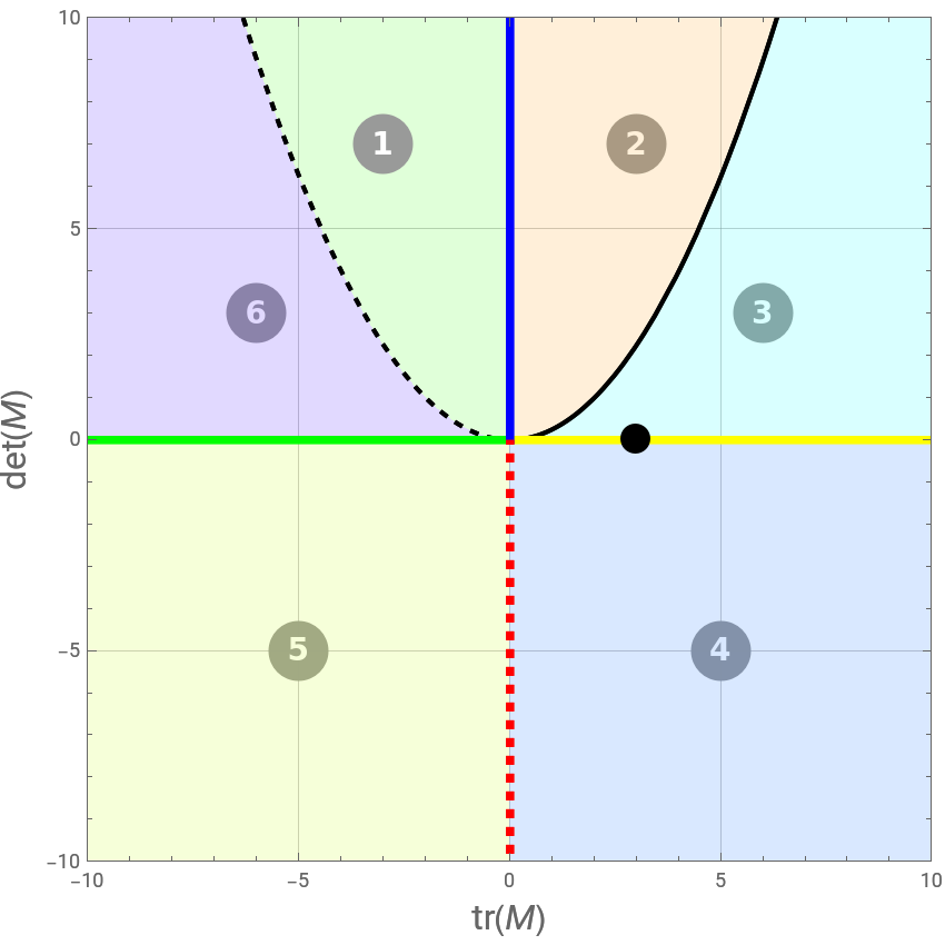
A plot of the curve obeying the equation is obtained if you select the stability character tab. This parabola is indicated in solid and dashed black curves for positive and negative values of , respectively.
Δ=0
tr(M)
The stability character of the steady-state is obtained by looking at the position of the black dot relative to the different colored regions (numbered 1–6).
region | eigenvalues | origin | tr(M) | M | Δ |
1 | complexconjugateswithnegativerealpart | asymptoticallystable | - | + | - |
2 | complexconjugateswithpositiverealpart | unstablespiral | + | + | - |
3 | realandpositive | unstableimpropernode | + | + | + |
4,5 | realwithoppositesigns | saddlepoint | - | + | |
6 | realandnegative | asymptoticallystableimpropernode | - | + | + |
green,-xaxis | …… | marginallystable | - | + | |
yellow,+xaxis | …… | unstable | + | 0 | + |
blue,+yaxis | pureimaginary | centerwithalimitcycle | 0 | + | - |
solidblackcurve | real,positive,andequal | unstablenodes | + | + | 0 |
dashedblackcurve | real,negative,andequal | stablenodes | - | + | 0 |
Permanent Citation
Permanent Citation
Housam Binous, Ahmed Bellagi
"Stability of a Linear Two-Dimensional Autonomous System"
http://demonstrations.wolfram.com/StabilityOfALinearTwoDimensionalAutonomousSystem/
Wolfram Demonstrations Project
Published: September 24, 2013