A tutorial
A tutorial
This effort was inspired by Jago Alexander’s YouTube video:
Here is a representation of the Gaussian integral. It appears as part of the Normal Distribution probability density function. It cannot be integrated by elementary methods. However, a method by Richard Feynman evaluates this integral . Since Mathematica reserves I for the Imaginary Number, we will name the indefinite integral “intgr.”
to
π
In[]:=
Remove["Global`*"]//Quiet(*removeallvariables*)
In[]:=
intgr=x
∞
∫
-∞
-
2
x
Out[]=
π
We notice that this is an even function of x.Thus it is symmetric.
In[]:=
Plot,{x,-3,3}
-
2
x
Out[]=
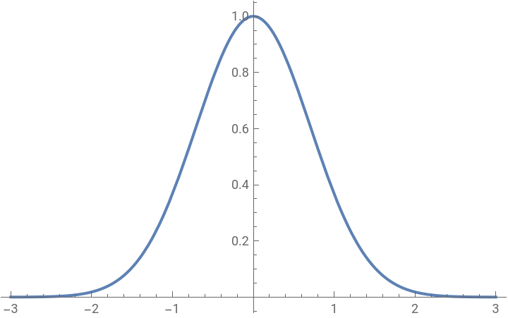
Therefore it can be expressed as twice half of it. We name half of it halfInt.
In[]:=
halfInt=x;GridPlot,{x,-3,0},Plot,{x,0,3}
∞
∫
0
-
2
x
-
2
x
-
2
x
Out[]=
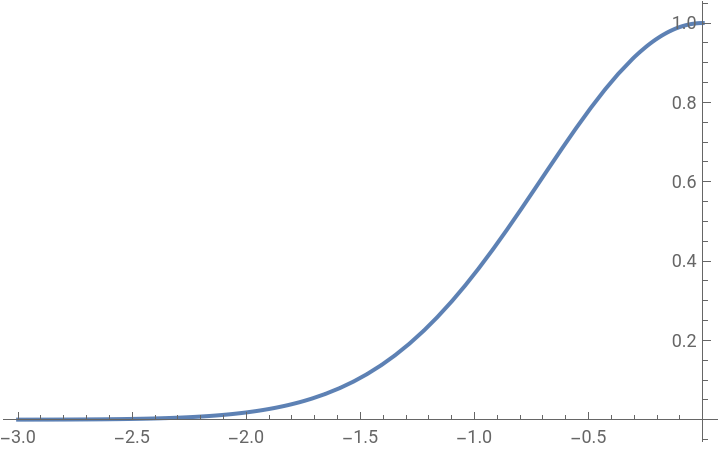
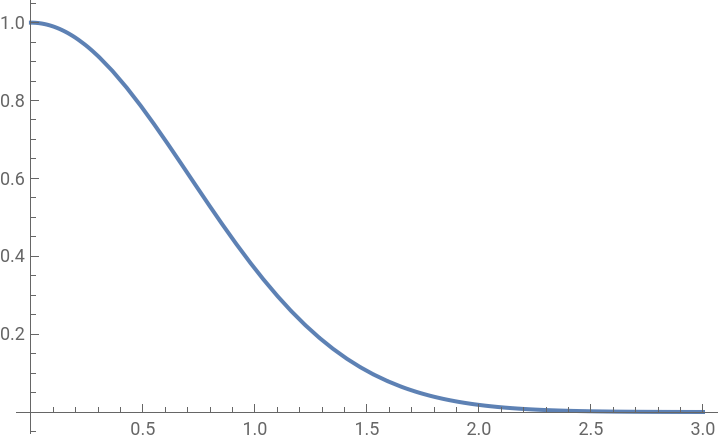
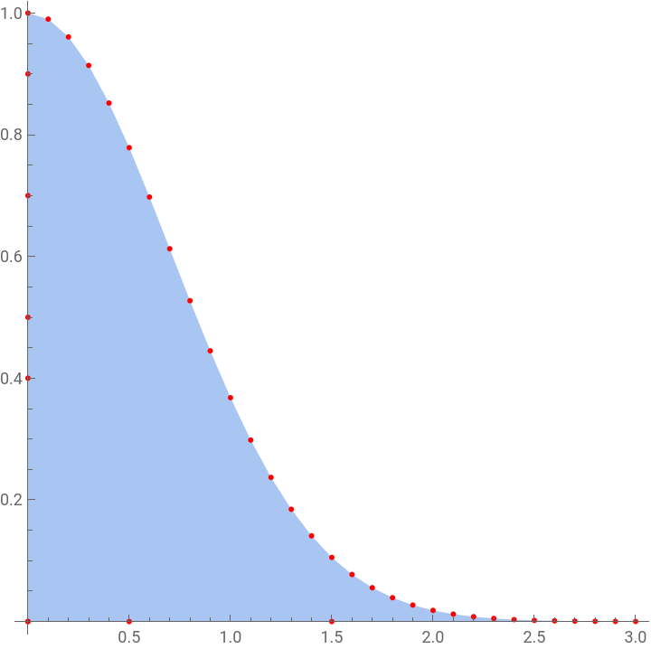
Mathematica has various ways to approximate the area under a curve. Here we use Region and the Wolfram Area function to obtain an answer which is just a number
In[]:=
pts=JoinTransposeRange[0,3,.1],Table,{x,0,3,.1},{{0,0},{.5,0},{1.5,0},{2.5,0}{0,.2},{0,.4},{0,.5},{0,.7},{0,.9}};
-
2
x
In[]:=
reg1=Region[Polygon[pts],Axes->True,AspectRatio->1];Show[reg1,Graphics[{Red,Point[pts]}]]polyAr=Area[reg1]
Out[]=
Out[]=
0.886022
We find this is very close to the evaluated answer, most of the difference being the area under the curve from 3 to infinity, a very small number.
In[]:=
N[halfInt]2*halfInt//N(*numericalvalueofhalfInt*2*)TrueQ[%==N[
π
]]halfInt-polyArOut[]=
0.886227
Out[]=
1.77245
Out[]=
True
Out[]=
0.000205306
We are also interested in the route that Wolfram takes to obtain the same answer. Unfortunately, Trace is not very helpful.
In[]:=
Tracex;%//TableForm
∞
∫
-∞
-
2
x
Out[]//TableForm=
|
| {x,-∞,∞} | ||||||||
∞ ∫ -∞ - 2 x | ||||||||||
| !True | False | ||||||||
∞ ∫ -∞ - 2 x | ||||||||||
π |
The FreeQ [ ] function is a check on pre-loaded function outcomes in the kernel. It returns “True” because the solution to this integral is known.
Feynman’s Method
Feynman’s Method
Key to Feynman’s method is the introduction of a parameter, , in both the numerator and denominator (harmless as a multiplier, as the ratio of two identical elements is just 1) and two changes of variable. Interesting things happen when we take the partial derivative of our new function, this time using “a” as our new dependent variable.
1+
2
x
In[]:=
f[a_]:=x;
∞
∫
0
-*(1+)
2
a
2
x
(1+)
2
x
In[]:=
f'[a]
Out[]=
In[]:=
∂
a
∞
∫
0
-*(1+)
2
a
2
x
(1+)
2
x
Out[]=
Mathematica is very particular. We get an answer only for certain conditions. In this case it is when the Real portion of is strictly positive.
2
a
In[]:=
AssumingRe[]>0,x
2
a
∂
a
∞
∫
0
-*(1+)
2
a
2
x
(1+)
2
x
Out[]=
-
a
-
2
a
π
2
a
Note we get the same answer when we take the partial derivative inside the integral
In[]:=
AssumingRe[]>0,x
2
a
∞
∫
0
∂
a
-*(1+)
2
a
2
x
(1+)
2
x
Out[]=
-
a
-
2
a
π
2
a
In[]:=
TrueQ[%==%%]
Out[]=
True
But, is all of this the same as our original integral?
In[]:=
TrueQx==-2ax==-2a*x
∞
∫
0
∂
a
-*(1+)
2
a
2
x
(1+)
2
x
∞
∫
0
-*(1+)
2
a
2
x
∞
∫
0
-
2
a
-
2
a
2
x
Out[]=
False
Only when we consistently restrict it to our assumption about the Real portion of .
2
a
In[]:=
TrueQAssumingRe[]>0,x==-2ax==-2a*x
2
a
∞
∫
0
∂
a
-*(1+)
2
a
2
x
(1+)
2
x
∞
∫
0
-*(1+)
2
a
2
x
∞
∫
0
-
2
a
-
2
a
2
x
Out[]=
True
Focussing on the last integral of the three above, we see it is just a distribution/expansion/rearrangement of the exponent term
Because the first term inside the integral on the left in the last expression does not depend on x it may be removed harmlessly to outside the integral
In[]:=
TrueQAssumingRe[]>0,-2ax==-2a*x==-2a*x
2
a
∞
∫
0
-*(1+)
2
a
2
x
∞
∫
0
-
2
a
-
2
a
2
x
-
2
a
∞
∫
0
-
2
a
2
x
Out[]=
True
In[]:=
-2a*x;%[[1]]
-
2
a
∞
∫
0
-
2
a
2
x
Out[]=
-
a
-
2
a
π
2
a
A reassignment and a change of variable. First make the ” term, an element to be squared, equivalent to *
"ax
2
)
2
a
2
x
In[]:=
TrueQ[==]
2
(ax)
2
a
2
x
Out[]=
True
Then assign u to a x, take its partial derivative and re-arrange to obtain a new definition for x (u must be cleared to avoid a conflict later)
In[]:=
u=ax;uxSolve[%==du,x][[1,1]]Clear[u];
∂
x
For the first limit, t→∞, all we care about is the numerator.
For the second limit, t→0, again only the numerator is important
Using hi as “half integral”
...this is the RHS of the equation...
... for which, this...
...is the LHS.
Here is half the integral...
Here is half the integral...
...and multiplied by 2 it is...
...the answer we seek.
A module to test performance
A module to test performance
Of course the next method is faster because Wolfram knows the solution for certain integrals, and this is one of them.
Two dimensional illustration of the above
Two dimensional illustration of the above
This section draws from insights provided in the vcubingx YouTube video here:
We will solve this by making it 3 dimensional which, unexpectedly, is actually easier. We again make use of the notation we used above
Or
The 3D illustration may be seen as an infinite number of cylinders, each of a smaller circumference reach a limit of zero at the top. Each cylinder may be seen as a cuboid, which when “unrolled” has a volume of
...simplifies the equation to
Or
The Chat-Enabled approach
The Chat-Enabled approach
Yet another approach, suggested by the Chat bot in version 14.1
This has been a curiosity for me, which I have now satisfied. As always, comments, enhancements, corrections, refinements are all welcome. One thing I searched for and could not find was the standard textbook notation for representing the mechanics of the Fundamental Theorem of Calculus which is a vertical bar with the upper and lower limits to the right of it indicating the lower evaluation should be subtracted from the upper evaluation. It does not appear in any Palette as far as I could find.
CITE THIS NOTEBOOK
CITE THIS NOTEBOOK
Feynman's technique to solve the Gaussian integral
by Roger J Brown
Wolfram Community, STAFF PICKS, September 15, 2024
https://community.wolfram.com/groups/-/m/t/3274410
by Roger J Brown
Wolfram Community, STAFF PICKS, September 15, 2024
https://community.wolfram.com/groups/-/m/t/3274410