As the aerospace industry shifts to long-term and deep-space missions, astronaut health has become a top priority. One particular negative effect of the space environment has been space-based radiation, which originates from trapped radiation from the Van Allen Belts, galactic cosmic rays (GCR), and solar particle events (SPE). Manned missions in Low-Earth Orbit (LEO) and beyond face the challenge of controlling astronaut radiation exposure by managing mission length and shielding. This research aims to evaluate levels of space-based radiation exposure for astronauts in different types of orbits and investigates the consequential medical effects of radiation. Along with that, the project centers specifically around the Van Allen Radiation Belts. The project utilizes three-dimensional visualizations to model the Earth, orbits, and radiation belts. Ultimately, these models aided in approximating sex-specific radiation exposures in any geocentric orbit. This data can be used by researchers to compare radiation exposure in a variety of orbits and flight paths in order to derive the corresponding health effects, allowing scientists to weight risk during mission planning phases in the interest of astronaut health.
Introduction
Introduction
Radiation in space is very different from the radiation humans experience on Earth. People experience much less radiation on the planet due to the magnetosphere and atmosphere, which deflect charged particles that often originate from deep space and solar flares. On Earth, people are more likely to experience radiation through radioactive gases and naturally occurring substances, which causes radiation to usually be targeted or limited to specific body parts. This fact is also reflected in existing radiation safety regulations for on-Earth radiation workers, but it is not the most realistic measure for astronauts. Instead, astronauts face three types of radiation: galactic cosmic rays (GCR), solar particle events (SPE), and trapped radiation. Generally speaking, GCRs and SPEs are largely unpredictable, and are the most dangerous types of space-based radiation. Galactic Cosmic Rays are composed of heavy ions created by high-energy events, such as supernova explosions, beyond the solar system. Solar Particle events are sudden bursts of highly energetic protons and heavy ions during solar flares and coronal mass ejections. Finally, this research is focused on the Van Allen Belts, which is rings of trapped radiation surrounding the Earth due to the same magnetic fields that protect people on ground.
For context, current space agencies such as NASA, JAXA, CSA, ESA, etc. use separate (but usually similar) measures and thresholds for radiation. The measurements and calculations in this project are based on the International Commission of Radiation Protection (ICRP), which is the largest governing body in radiation regulation. Overall, mild and recoverable effects of radiation include changes in blood, nausea, diarrhea, skin rash etc. Radiation may also cause radiation sickness, acute radiation syndrome (ARS), cataract development, tumor necrosis, and in severe cases, central nervous system damage, cancer, or death. However, these symptoms are mainly dependent on the duration and intensity of the exposure, the type of radiation, solar weather conditions, and the clinical profile of the astronaut. Additionally, the microgravity environment might worsen these effects by weakening the immune system or limiting medical interventions while in space. Thus, research on space-based radiation and development of flight path optimization are essential to ensure the safety of astronauts and the growth of the aerospace industry.
For context, current space agencies such as NASA, JAXA, CSA, ESA, etc. use separate (but usually similar) measures and thresholds for radiation. The measurements and calculations in this project are based on the International Commission of Radiation Protection (ICRP), which is the largest governing body in radiation regulation. Overall, mild and recoverable effects of radiation include changes in blood, nausea, diarrhea, skin rash etc. Radiation may also cause radiation sickness, acute radiation syndrome (ARS), cataract development, tumor necrosis, and in severe cases, central nervous system damage, cancer, or death. However, these symptoms are mainly dependent on the duration and intensity of the exposure, the type of radiation, solar weather conditions, and the clinical profile of the astronaut. Additionally, the microgravity environment might worsen these effects by weakening the immune system or limiting medical interventions while in space. Thus, research on space-based radiation and development of flight path optimization are essential to ensure the safety of astronauts and the growth of the aerospace industry.
Modeling the Van Allen Belts
Modeling the Van Allen Belts
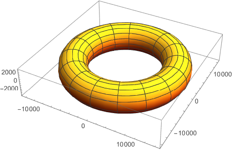
The Van Allen radiation belts encompass two torus-shaped rings of radiation. The inner belt is composed of trapped protons from Galactic Cosmic Rays and is located at an altitude ranging from 1,000-12,000 km above the Earth’s surface. Unlike the outer radiation belt, the inner belt stays relatively constant in size and intensity.
3D Parametric Plot of torus, representing the inner belt
ParametricPlot3D[{(10500+3000Cos[v])Sin[u],(10500+3000Cos[v])Cos[u],3000Sin[v]},{u,0,2Pi},{v,0,2Pi},ColorFunction->"SolarColors"]
Out[]=
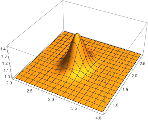
The inner radiation belt also includes a unique phenomenon called the South Atlantic Anomaly (SAA). This is caused by a weak spot on the Earth’s magnetic field, leading to a small section of the inner radiation belt to reach closer to the Earth’s surface. The SAA is a relevant risk for manned missions in LEO, which often intersect with the anomaly. The measurements used below to create the anomaly are only estimations, due to the fact that there is a lack of data regarding the size and shape of it.
Define the anomaly as a gaussian surface:
In[]:=
anomalyFunction[v_,u_]:=(1+Exp[-((u-Pi/1.8)/0.3)^2]*Exp[-((v-(2.916)))^2/0.04]*0.45);
3D Plot of the South Atlantic Anomaly (SAA)
Plot3D[anomalyFunction[v,u],{v,2,4},{u,Pi/1.8-2*Pi/3/2,Pi/1.8+2*Pi/3/2},PlotRange->All]
Out[]=
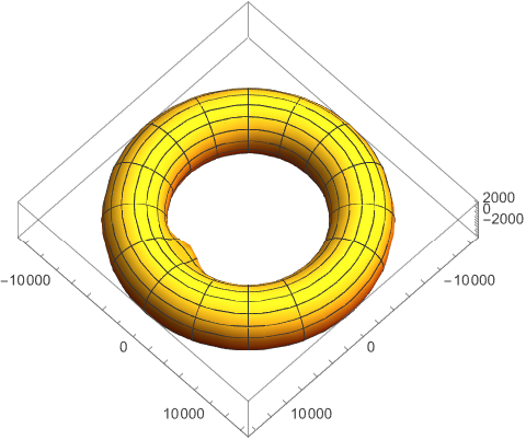
A set of localized rules were used to create and integrate the anomaly into the belt, but only in a specific section so as to not interfere with the original belt function.
Define the inner belt function:
In[]:=
innerBeltAnomaly[r1_,r2_,u_,v_]:={((10500+r1)+(3000+r2)Cos[v])Sin[u],((10500+r1)+(3000+r2)Cos[v])Cos[u],(3000+r2)Sin[v]};innerBeltAnomaly[r1_,r2_,u_,v_]/;And[Between[v,{1.417,3.416}],Between[u,{0.746,2.745}]]:={((10500+r1)+anomalyFunction[v,u]*(3000+r2)Cos[v])Sin[u],((10500+r1)+anomalyFunction[v,u]*(3000+r2)Cos[v])Cos[u],anomalyFunction[v,u](3000+r2)Sin[v]};
3D Parametric Plot of torus with a conditional function to create a localized anomaly:
innerbeltplot=ParametricPlot3DinnerBeltAnomaly[0,0,u,v],{u,0,2Pi},{v,0,2Pi},
Out[]=
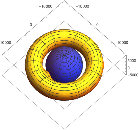
What does this look like at scale? Here is a three-dimensional model of the inner Van Allen Belt with its corresponding anomaly, along with the Earth. This model also includes the orbit of the International Space Station (ISS)
Define the model of the Earth:
In[]:=
earth=ParametricPlot3D[{6378Cos[u]Sin[v],6378Sin[u]Sin[v],6357Cos[v]},{v,0,Pi},{u,0,2Pi},PlotStyle->FaceForm[Lighter@Blue]];
3D Model of the Earth, Inner Van Allen Belt, and the orbital path of the International Space Station (ISS)
Show[earth,innerbeltplot,PlotRange->All,ViewPoint->{1000,1000,2500}]
Out[]=
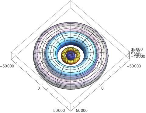
The outer Van Allen Belt is composed mainly of electrons generated by solar particle events, and ranges from 15,000-25,000 km. However, solar activity may cause this range to reach up to 60,000 km. Therefore, an extended radiation belt was added to account for slight trapped radiation past the outer belt. It is important to keep in mind that there is radiation everywhere in space, but that trapped radiation exists specifically in the Van Allen Belts and surrounding areas.
Definition of the outer belt:
In[]:=
outerBelt=ParametricPlot3D[{(28000+9500Cos[v])Sin[u],(28000+9500Cos[v])Cos[u],9500Sin[v]},{u,0,2Pi},{v,0,2Pi},ColorFunction->"DeepSeaColors"];
Definition of the extended belt:
In[]:=
extendedBelt=ParametricPlot3D[{(43000+9500Cos[v])Sin[u],(43000+9500Cos[v])Cos[u],9500Sin[v]},{u,0,2Pi},{v,0,2Pi},ColorFunction->"PearlColors",PlotStyle->Opacity[0.5]];
3D Parametric Plot of inner belt, outer belt, extended belt and the Earth for reference
Show[innerbeltplot,outerBelt,extendedBelt,earth]
Out[]=
Modeling Geocentric Orbits
Modeling Geocentric Orbits
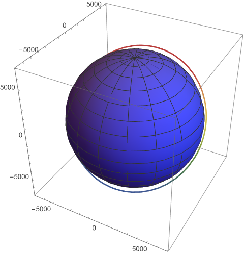
The aerospace industry has many standard orbits with unique uses. All orbits were defined computationally by plotting the orbital radius, inclination, and eccentricity. This accounts for the distance from the center of the Earth to the orbit, the angle of the orbit, and how elliptical or circular it is on a scale of 0-1. Here is once again the example of the orbit of the ISS:
Define a general function that will be used to generate the orbits:
In[]:=
orbitFunction[orbitradius_,inclination_,eccentricity_:0,t_]:=({((orbitradius)/(1+eccentricity*Cos[t]))*Cos[t],((orbitradius)/(1+eccentricity*Cos[t]))*Sin[t]*Cos[inclinationDegree],((orbitradius)/(1+eccentricity*Cos[t]))*Sin[t]*Sin[inclinationDegree]});
Plot the orbital path of the International Space Station using average orbital radius, inclination, and eccentricity:
In[]:=
issPath=ParametricPlot3D[orbitFunction[6796.167,51.64,0.007,t],{t,0,2Pi},ColorFunction->"DarkRainbow"];
3D Parametric Plot of the ISS path and the earth .
Show[earth,issPath]
Out[]=
Low Earth Orbit (LEO) is the most common orbit ranging from 100-2,000 km, and tends to cross the SAA. LEO contains the ISS and many other spacecraft that center around scientific research and observation. Very Low Earth Orbit (vLEO) ranges from 100-450 km, and is the closest orbit to Earth, often used for high-quality imaging. Medium Earth Orbit (MEO) spans from 2,000-35,786 km, and houses navigation systems. Geostationary Orbit (GEO) is exactly at 35,786 km, thus matching the Earth’s rotation and remaining in one position. Polar orbits have similar altitudes as LEO, and have inclinations at around 90 degrees. Lastly, sun-synchronous orbit sits at 600-800 km, and is slightly higher than 90 degrees, allowing satellites to match the Earth’s rotation around the Sun.
3D Parametric Plots of Polar orbit, LEO, GEO, MEO, vLEO, and Sun-Synchronous orbit
In terms of radiation exposure, Medium Earth Orbit (MEO) is located directly within the Van Allen Belts. Although Geostationary orbit is larger, it sometimes has a higher altitude than the radiation belts. Lower orbits such as LEO, vLEO, polar, and Sun-synchronous often cross the South Atlantic Anomaly and perhaps the inner belt. Despite the fact that most manned missions happen in lower orbits, the LEO environment is becoming more congested due to orbital debris. These issues in space traffic management and space domain awareness may lead to industry shifting to less common orbits such as MEO and beyond.
Helper function to plot the orbits:
Definition of orbits:
3D Parametric Plots of Polar orbit, LEO, GEO, MEO, vLEO, and Sun-Synchronous orbit:
Quantifying Distance and Time in “Danger Zones”
Quantifying Distance and Time in “Danger Zones”
The method to calculating a specific dose of radiation an astronaut would experience in a specific orbit is to determine how long the astronaut is spending within the radiation belts, or “danger zones”. The first step to this process is to plot both the orbit and the belts, and then extract the points (if any) that intersect between the two values. In this project, both the belts and the user-inputted orbit were split into thousands of small sections. These sections were then compared to find matching coordinates, and were then plotted to create visualizations. Using list manipulation, matching points between the belt and orbit were selected and then combined to calculate the total Euclidean distance of matching coordinates. This distance measurement was then divided by the orbital velocity of the orbit to then output the time spent within the belt. This process was executed separately for both the inner and outer belt, due to the distinctions in the composition and intensity of each belt.
Finding the Intersection
Finding the Intersection
First, the orbital trajectory function and the belt definitions were used to find the sections of the orbit that happen to be inside the belt, which will later on help to calculate dosage exposure.
3D Parametric Plot of an example orbit
The inner belt and the example orbit first need to be sampled so the points can be used to check whether they are inside the danger zone .
Sample the inner radiation belt:
Create a function to sample any orbit:
Define an example orbit
Now I need a function to calculate the baseline angle between the orbit and the belt using the vector dot product. However, because of the ambiguity of the Cosine in the first and fourth quadrant the resulting angle will need to be adjusted when needed.
Function to calculate the angles between points in the XY projection:
Function to fix the angle ambiguity:
Another important fact is that the Van Allen Belts rotate in synchrony with the Earth, while the orbit remains in a fixed location. This phenomenon would be hard to simulate as it is, so instead the orbit was rotated rather than the belt. This action outputs the exact same values as the real life events. Rotations in the YZ plane were performed to place points in the same plane as the belt, in order to simplify the calculation. The rotation trajectory function rotates each orbit point across the belt, flips the signs when necessary, and accounts for a slight adjustment in 90 degree orbits. When an orbit has exactly a 90 degree inclination, it will often have the wrong rotational direction. Thus, the condition below does an extra rotation in case it is a 90 degree orbit, such as the case for the example.
Function to rotate points onto the YZ plane:
Once the points were rotated, these values were plotted in 3D. The graphic below has a cross-section of the inner belt and all of the orbital points. The orbital points are in red along with a black dot that represents the center of the Earth. Each orbital point also contains its angle.
Helper function to visualize the rotation
After identifying the matching points between the inner belt and the theoretical orbit, list manipulation was used to save only the desired points. A function was created to identify each orbital point by adding “True” if it is within the belt, and “False” if it lies outside of the inner belt.
Define the boolean region for checking if a point is inside:
Function that classifies the sampled points:
Below is an alternate method to visualize the intersection between the inner Van Allen radiation belt and the example orbit. The cross-section of the inner belt is plotted in 3D, along with a color-coded orbit. Points that intersect with the inner belt are marked in red, along with the blue points on the orbit. Green points are parts of the orbit that sit outside of the radiation belt.
3D Graphic of inner belt cross-section and color-coded orbital points
Check if a point is in or out of the inner belt:
3D Graphic of inner belt cross-section and color-coded orbital points
Time Calculation
Time Calculation
The next step was to use only the points within the belt and then partition the values into lists of three elements.
Select only true coordinates and partition into list into groups of three elements.
From there, a function that inputs the coordinates within the belt calculates the Euclidean Distance between each point and then adds them together for the total distance spent in the inner radiation belt.
Function that totals the Euclidean distance between the inner coordinates
Once the distance is calculated, this value must be used to calculate the orbital velocity. The orbital velocity is how fast a spacecraft travels in a path, in this case it will be measured in kilometers per hour. To do this, the values must be multiplied by 3,600. The inputs for this orbit are the orbital radius, the distance from the center of the Earth to the orbit, and the semi-major axis, the average distance between an orbiting object and the body it orbits. This is necessary to account that the Earth is not perfectly circular, and neither are most orbits. This measure will then contribute to calculating the total time in hours that was spent within the inner radiation belt.
Earth gravity parameter and orbital velocity calculator in kilometers per hour:
Orbital velocity function for example orbit:
Both the orbital velocity and distance traveled within the belt were used to calculate the total time in hours spent in the inner radiation belt using the following function.
Calculate the time for one orbital period by dividing orbital velocity and distance:
The output of the function above means that an astronaut traveling this theoretical orbit would have spent approximately 2.38718 hours within a danger zone, that being the inner radiation belt. This number will then be used to calculate the total effective dose of radiation in this specific example orbit.
Outer Orbit Intersection
Outer Orbit Intersection
After calculating the total time spent within the inner belt, one must repeat this process for the outer belt. In this section, a different example will be used to make the outer belt intersections clear. The function below contains the orbital radius, inclination, and eccentricity of the new orbit and has been split into sections 0.1 km each.
Function of example orbit that intersects with the outer belt split into sections 0.1 km each:
Similarly to the inner belt, the outer belt must be split into tiny sections of 0.1 km.
Functions that defines the coordinates of the outer belt:
Split the outer belt into sections 0.1 km each:
One difference between the functions used to calculate distance for the inner belt versus the outer belt is that the values change. In the rotation trajectory function, the value of 13,500 km was used since it is the farthest point of the inner belt. In this case, the point 37,500 km will be used, as it is the farthest point of the outer belt.
Return the farthest point of the outer belt in kilometers:
Subsequently, each point in the example orbit will be rotated around the outer belt. As stated previously, this is the opposite to what happens in the physical world, but it yields the exact same outputs. Thus, the sign of the points will be flipped to ensure a continuous orbit. Orbits with an inclination of 90 degrees, such as this example orbit, need an extra adjustment so as to maintain the correct rotational direction.
Rotate the orbital points by 180 degrees and correct rotational direction in 90 degree orbits:
After retrieving the rotated points, these values were then displayed in a 3D plot. Here, each orbital point is visible along with each angle. Additionally the cross-section of the outer belt and its intersecting points are shown.
Function of 3D Plot for rotated orbital points and cross-section of outer radiation belt:
3D Plot of example orbital points, angles, and intersections with outer belt:
Another method of visualization that was conducted was a 3D graphic of the cross-section of the outer belt with the intersecting points marked in red. The model also contains the rotated orbit with points that contact the belt in blue and points outside of the belt in green.
Once the example orbit points have been intersected with the outer orbit, the time calculation process must be repeated. This first function labels a coordinate with “True” if it intersects with the outer belt or “False” if it falls outside of the outer belt.
Check if orbital points are in or out of the outer belt by stating “True” or “False”:
Label the example orbital points by their position relative to the outer belt:
3D Graphic outer belt cross-section and color-coded example orbit:
Outer Orbit Time Calculation
Outer Orbit Time Calculation
After all points have been classified, the “True” points were extracted. Using list manipulation, the string “True” was removed and the points were split into 3D coordinates of three elements.
Select the true points, remove the string “True”, part the list into groups of three values:
Next, the total Euclidean distance was calculated between the points and then combined to output the total distance traveled within the outer belt.
Calculate the total Euclidean distance between the intersecting orbital points:
Total Euclidean distance of example orbit within outer radiation belt:
To output the total time spent within the danger zone, the orbital velocity was also calculated. This function is the same as what was used earlier with the inner belt, but with the values of the new example orbit.
Calculate the orbital velocity of the example orbit:
With the orbital velocity and total distance values, the time spent within the danger zone was calculated in hours. This number will later be used to calculate the effective dose of radiation by combining the hours spent within the inner belt and outer belt.
Function that divides distance by orbital velocity to output time:
Total time spent in the outer orbit danger zone for example orbit:
Radiation Medicine
Radiation Medicine
Radiation is one of the most threatening properties of space. High-energy activity such as supernovae explosions from light years away and solar flares can have detrimental impacts on astronauts. Along with that, some effects of ionizing radiation such as central nervous system deterioration are not well studied. Space agencies, international organizations, and regulation committees have to adapt to new scientific discoveries of space-based radiation.
Radiation Symptoms
Radiation Symptoms
Generally, radiation may cause skin rashes, acute radiation syndrome, radiation sickness, etc. Severe cases usually relate to heritable genetic changes, cancer, degenerative tissue effects, cataract development, sterility, tumor necrosis, and central nervous system decrements. These effects vary drastically based on the duration and intensity of the exposure. Additionally, extra-vehicular activity (EVA) or spacewalks cause a major influx in radiation exposure for astronauts. Therefore, shielding and mission planning are important factors to radiation protection.
Radiation safety organizations classify the effects of ionizing radiation as deterministic or stochastic. Deterministic effects increase in severity with higher doses of radiation, and can include most of the symptoms mentioned previously. Milder symptoms are usually up to 0.7 Sv (Sieverts), and anything higher than that begins to be severe. On the other hand, stochastic effects can happen at any level of radiation and are the most dangerous symptoms. This includes cancer and genetic changes due to long-term exposure to ionizing radiation. Furthermore, some of these mutations will be expressed in offspring through mutations in gametes.
Radiation safety organizations classify the effects of ionizing radiation as deterministic or stochastic. Deterministic effects increase in severity with higher doses of radiation, and can include most of the symptoms mentioned previously. Milder symptoms are usually up to 0.7 Sv (Sieverts), and anything higher than that begins to be severe. On the other hand, stochastic effects can happen at any level of radiation and are the most dangerous symptoms. This includes cancer and genetic changes due to long-term exposure to ionizing radiation. Furthermore, some of these mutations will be expressed in offspring through mutations in gametes.
Radiation Thresholds Globally
Radiation Thresholds Globally
All space agencies have radiation thresholds for their astronauts, which may extend from 30 days to career-long limits. Many agencies follow the International Commission of Radiation Protection (ICRP); meanwhile, some agencies adjust those values for their astronauts. Career radiation thresholds range from 600-1,000 mSv and may take into account other values, similar to how NASA requires the cancer mortality rate to be under 3%. Unfortunately, some agencies still uphold the same thresholds and regulations for astronauts as for on-Earth radiation workers. However, this is highly unrealistic to the space environment due to the fact that radiation exposure is unlikely to be as targeted and spatially limited as it is on Earth.
As mentioned, deterministic effects worsen with higher levels of radiation while stochastic effects do not have a linear ranking of effects. Due to this fact, stochastic effects do not have thresholds and use the Linear Non-Threshold Model. This model signifies that the risk of cancer and heritable diseases is possible at any dose of radiation.
As mentioned, deterministic effects worsen with higher levels of radiation while stochastic effects do not have a linear ranking of effects. Due to this fact, stochastic effects do not have thresholds and use the Linear Non-Threshold Model. This model signifies that the risk of cancer and heritable diseases is possible at any dose of radiation.
Effective Dose Function
Effective Dose Function
There are many ways to quantify radiation exposure. The most objective measure used is the absorbed dose. This is the amount of energy absorbed by some material, such as the human body, in Grays (Gy). This absorbed dose is then multiplied with a quality factor (Q Factor) to determine the biological damage of the radiation. This is because different types of radiation, even at equivalent absorbed doses, have different effects. The quality factor is a number assigned to different types of charged particles to quantify its intensity. More complex equations use the radio-biological effectiveness measure (RBE). This is the ratio of the absorbed dose of low-Linear Energy Transfer (LET) needed to cause the same effect as high-LET radiation. LET is the average energy released per unit length of track. Low-LET is comparable to gamma rays or X-rays.
After the absorbed dose is multiplied by the quality factor, the dose equivalent is evaluated. The dose equivalent is how much biological damage the radiation has caused, and is often combined with patient information such as sex, age, health status, etc. to compute an accurate measurement for the specific astronaut. However, this measurement is nearly impossible to replicate, as the patient information factors are subjective decisions made by medical experts. The last measurement for radiation exposure is the effective dose. The effective dose uses a tissue weighting factor that represents the sensitivity of an organ to radiation, and multiplies it by the dose equivalent. The sum of effective doses for all organs is the total effective dose for an astronaut.
After the absorbed dose is multiplied by the quality factor, the dose equivalent is evaluated. The dose equivalent is how much biological damage the radiation has caused, and is often combined with patient information such as sex, age, health status, etc. to compute an accurate measurement for the specific astronaut. However, this measurement is nearly impossible to replicate, as the patient information factors are subjective decisions made by medical experts. The last measurement for radiation exposure is the effective dose. The effective dose uses a tissue weighting factor that represents the sensitivity of an organ to radiation, and multiplies it by the dose equivalent. The sum of effective doses for all organs is the total effective dose for an astronaut.
The function below takes in the time in hours spent in the inner belt, the time spent in the outer belt, and the sex of the astronaut as a string. The function takes the time and multiplies it by the average amount of radiation an astronaut is exposed to in one hour in space. This is then multiplied by the quality factor, which is 2 for protons and 1 for electrons. Lastly, it multiplies by the sum of all organ weighting factors depending on the sex of the astronaut.
Radiation calculation in Sieverts (Sv) using time in danger zones and sex-specific dose equivalence:
Interestingly, women have higher effective doses of radiation than men with the same absorbed dose. This is because women have more organs than men, which means that the total sum of the organ weighting factors is larger than that of men.
Comparison of effective radiation dose of men vs. women:
The effective dose function can now calculate how much radiation an astronaut would theoretically be exposed to in both of the example orbits. For the first example, the time spent within the inner belt had been 2.38718 hours.
Effective Dose radiation in Sieverts of example inner belt orbit:
For the second orbit example, the time spent within the outer belt was 6.29688 hours.
Effective Dose radiation in Sieverts of example outer belt orbit:
Conclusion
Conclusion
In conclusion, this research focused on creating a process to calculate the total biological damage of space-based trapped radiation on astronauts. Three-dimensional models of the Earth, equator, and orbits were created to simulate the space environment. Then, the inner and outer belt were modeled using torus shapes, along with the South Atlantic Anomaly (SAA) and empty space for the slot. After that, multiple functions were created to split orbits and belts into small sections to allow for comparison. Orbits were rotated to be on the same plane as the belt, and orbital points that intersected with the belt were extracted. These points were then used to determine the total time spent in a danger zone. This time measurement in hours was then used to calculate the effective dose. This dose quantity accounts for sex-specific biological differences and factors in each organ individually, along with the quality factor (Q factor) between the intensity of protons and electrons. The total effective dose for a specific orbit can be used to estimate the radiation effects for one orbital period. Additionally, this algorithm can be used to compare multiple orbits, and decide which would be best for a specific mission. By optimizing mission planning and continuing space-based radiation research, the aerospace industry can ensure occupational safety for astronauts.
Future Directions
Future Directions
This research has endless ways to improve accuracy and optimize radiation dose calculations. Naturally, radiation research holds some uncertainty due to the lack of data. Most information on radiation effects are derived from astronauts, who are a very small percentage of the population and have exceptionally good health status. Along with that, due to time constraints, the South Atlantic Anomaly (SAA) was not factored into the effective dose. Although the effective dose takes into account tissue-based weighting factors, it does not use patient data such as age and health status. These numbers are hard to replicate and would have to be estimated using large datasets and patient data. Future extensions will add the SAA levels of radiation, as it is essential for accurate radiation measures for Low-Earth orbit especially. Additionally, calculations and models will be refined to be as accurate as possible, and orbits will be compared to later determine which orbits pose the biggest threats to high radiation exposure.
References
References
Chancellor, J. C., Scott, G. B. I., & Sutton, J. P. (2014). Space radiation: The number one risk to astronaut health beyond low earth orbit. Life : Open Access Journal, 4(3), 491–510. https://doi.org/10.3390/life4030491
Nasa—Space radiation analysis group (Srag) web site. (n.d.-a). Retrieved July 9, 2026, from https://srag.jsc.nasa.gov/SpaceRadiation/Why/Why.cfm
Nasa—Space radiation analysis group (Srag) web site. (n.d.-b). Retrieved July 9, 2026, from https://srag.jsc.nasa.gov/spaceradiation/faq/faq.cfm
Physics, V. (2021, April 21). Deterministic vs. Stochastic effects: What are the differences? Versant Medical Physics and Radiation Safety. https://www.versantphysics.com/2021/04/21/deterministic-vs-stochastic-effects/
Radiation weighting factors. (2019a, August 15). ENS. https://www.euronuclear.org/glossary/radiation-weighting-factors/
Radiation weighting factors. (2019b, August 15). ENS. https://www.euronuclear.org/glossary/radiation-weighting-factors/
Tissue weighting factor. (2020, November 17). University of Groningen. https://www.rug.nl/education/courses/other-education/radiation-protection/a-z/a-z-data/tissue-weighting-factor
What are the Van Allen Belts and why do they matter? - NASA Science. (2023, February 10). https://science.nasa.gov/biological-physical/stories/van-allen-belts/
Acknowledgements
Acknowledgements
I want to take the time to thank my mentor, Rafael Caballero, for all of his help and support. His physics knowledge and coding skills were essential for the execution of this project. I am also very grateful for my advocate, William Choi-Kim, for helping me develop my coding skills before this project and checking in during my progress. I also want to thank Joseph Brennan, an astrophysicist, who offered his support and encouraged the idea. Thank you to our lead TA Anne Shuai for checking on me every day and asking thought-provoking questions. Thank you to Kaavya, Eileen, Aanya, and Averyl for being my dearest TAs. I am also extremely grateful for my dorm room (Sophia, Natalie, Annabella, Acadia, Ivy, Ananya, Estella, Ava) who helped me, consoled me, and supported me throughout this project. Thank you to the Wolfram Summer Research program directors (Eryn, Rory, Megan), mentors, and students for all of your support!
Last, but not least, I’d like to thank Stephen Wolfram for suggesting the idea in the first place. He came up with a project that beautifully combined my interests, and I had a blast conducting this research.
CITE THIS NOTEBOOK
CITE THIS NOTEBOOK
Calculating orbit-specific doses of space-based trapped radiation for astronaut protection
by Eva Estrada
Wolfram Community, STAFF PICKS, July 9, 2026
https://community.wolfram.com/groups/-/m/t/3753930
by Eva Estrada
Wolfram Community, STAFF PICKS, July 9, 2026
https://community.wolfram.com/groups/-/m/t/3753930