Introduction
Introduction
If a Wolfram Model is to accurately represent a model of the world, then it must reproduce known physics in the appropriate limits. One observable physical phenomenon that was recently directly confirmed is the existence of gravitational waves. Therefore, it seems reasonable to search for models that accurately reproduce gravitational wave-like effects in the large scale limit. In general relativity space is no longer treated as an unchanging rigid background, but rather as a dynamic manifold that can change over time. Space and time are dynamic quantities that are perturbed by the presence of mass and energy. A consequence of this phenomenon is the fact that space itself can be stretched and squeezed by the motion of matter and ripples can form in spacetime that affect the distances between freely falling test particles. The graphic below shows a somewhat exaggerated depiction of the effect of these test particles when a gravitational wave is incident into the page. On one axis, distances are stretched, while in the orthogonal direction, distances are compressed by a corresponding amount.
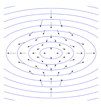
The aim of this project is to find discrete analogs of these gravitational waves in Wolfram Models by investigating what happens when the spacetimes of these models are perturbed. First a suitable manifold must be found to do the perturbation. After this is done, the perturbation must be formulated in a way that can produce relevant phenomena. Then, we must find a relevant metric to measure physical distances in order to probe the effects the perturbation has on the spacetime metric. The hope would then be to find variations in distances along orthogonal directions transverse to a propagating wave that would be anti-correlated with each other.
Finding suitable manifolds
Finding suitable manifolds
The first thing that was done was to find rules that produced manifold-like structures. There was no real systematic way of doing this, so I just looked at rules in the Registry of Notable Universe Models for some notable ones that intuitively looked like manifolds. The following figure represents the spatial hypergraphs of manifolds that I analyzed throughout this project, labeled by their short code number:
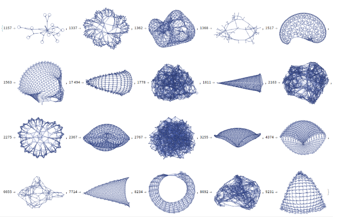
The ones that I found notable can be roughly divided into three categories based on their causal graph:
Sequentially growing structures,
Sequentially growing structures,
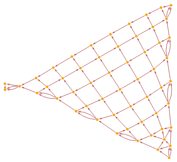
tree like structures,
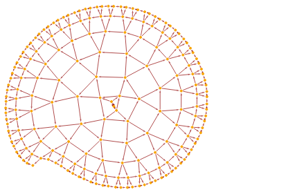
and stochastic structures.
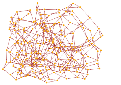
All of these rules were also space growing structures.
Perturbing Wolfram Model wm7714
Perturbing Wolfram Model wm7714
The first manifold that was analyzed was wm7714, as this produced a nice simple 2D spatial manifold and represented a nice testbed to develop tools for perturbations which could then be deployed on more complicated models. In this model, both the spatial and causal hypergraph look similar and this is no coincidence, since each generational time step represents a single event corresponding to a single addition of a spatial hyperedge.
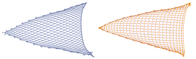
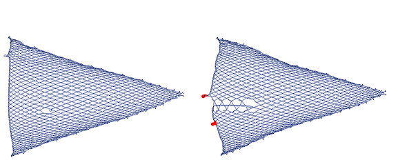
The next thing to do was decide how to implement the perturbation onto the Wolfram Model. At first, adding the perturbation as a rule was tried, but this seemed to disturb the causal graph in unnecessary ways. Therefore after talking to Max Piskunov, I decided to split up the evolution into unperturbed and perturbed graphs, using the final state of the unperturbed graph as a starting point to add perturbations. The following represents the first attempt at making a perturbation in the spatial hypergraph. I simply picked an edge close to the center and replaced it with another edge that matched the LHS of the rule in question to guarantee that this perturbation would have an effect on the graph. It turns out that this perturbation in effect travels downwards along the direction of the most recently stitched edges and leaves a ripple like pattern in its wake.
Stitching together the perturbed causal graph
Stitching together the perturbed causal graph
The next thing to do was to try to analyze the causal graph. However, since the perturbation was done by splitting up the evolution, the causal graph was not preserved and I had to create a function to stitch together the causal graphs:
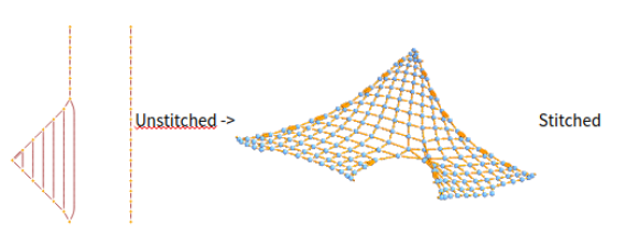
The left graph represents the portion of the causal graph after taking the initial spatial hypergraph, perturbing it, and then using the final state as an initial condition to be evolved further. The right graph represents the entire causal graph including the causal graph associated with the initial spatial hypergraph. After stitching together the graphs, it is clear that the causal graph splits where the perturbation occurs, which would not have been as obvious without combining the causal graphs.
In further detail, I created the following function, PerturbedCausalGraph, which takes two arguments, the unperturbed and perturbed WolframModelEvolutionObjects:
In further detail, I created the following function, PerturbedCausalGraph, which takes two arguments, the unperturbed and perturbed WolframModelEvolutionObjects:
PerturbedCausalGraph[wm0_WolframModelEvolutionObject,wm1_WolframModelEvolutionObject]:=
The key point here is that each event is associated with an “edge creator event” and an “event destroyer event”. By keeping track of these indices, we can reconstruct which edges are associated with each causal edge. Since the edges associated with the final state of the initial evolution object do not have “edge destroyer events” we can transfer these over to the perturbed object and continue the causal graph evolution.
In essence, to track differences between the two objects, I used the function SequenceAlignment to track changes in the edges of the initial state of the perturbed object and final state of unperturbed object:
This allows us to track regions of insertions, deletions, and replacements. The ordering of edges is important here, so shuffling the edges will result in loss of information in the causal graph.
Link to ResourceFunction: https://www.wolframcloud.com/obj/williamyam/DeployedResources/Function/PerturbedCausalGraph
Link to ResourceFunction: https://www.wolframcloud.com/obj/williamyam/DeployedResources/Function/PerturbedCausalGraph
Measuring Distances
Measuring Distances
At first I tried measuring distances between randomly chosen vertices on the graph that were not affected by the perturbation. The following represents two such points and the shortest path between them highlighted in red before and after the perturbation:
After playing around with the graphs, I found that for most growing graphs, I did not have to worry about disappearing vertices, and so I decided not to filter out any vertices when deciding which nodes would be the test points. Although, I found an exception to the rule of vertices being preserved in rule wm1811.
In the case where vertices are not preserved, one must then keep track of their replacements when tracking coordinates, but fortunately this did not apply for the other manifolds in question. However, for further analysis, a procedure must be developed to keep track of coordinates in the case where vertices do disappear.
Reformulating the perturbation and refining distance measurements
Reformulating the perturbation and refining distance measurements
Once the procedure for measuring distances was decided, I went back to reformulate the perturbation so that it always started at the graph center and also made its size vary as a function of radius from the graph center. I also made it so the perturbation consisted of self loops in order to match as many rules as possible. These perturbations only add edges to the graph, they do not add vertices, nor delete vertices, nor delete edges.
Building a gravitational wave detector
Building a gravitational wave detector
Looking for a better manifold: wm6655
Looking for a better manifold: wm6655
From the rules studied so far, most of the behavior has been rather non-gravitational wave-like. I suspect this is because the rules that have been investigated have mostly simple behavior and do not sample the spatial hypergraph thoroughly enough to notice any particular perturbation. In effect, one expects the perturbation to have wave-like behavior, which requires the effect to propagate throughout the spatial hypergraph, but this can only be the case if most of the spatial hyperedges are responsive to the perturbation to carry information away from it. One rule that was suggested by Stephen Wolfram was the 2.7 dimensional rule wm6655 which is known to have stochastic behavior.
The hope would be for this rule to be sufficiently random enough such that more interesting behavior would follow after a perturbation, and it seems like there is at least stochastic behavior. We can see this from the various plots of distances and strain vs time. In this case, the strain is no longer monotonic, but now has fluctuations as well. Due to the stochastic nature of the graphs, it is hard to analyze the differences in the causal graphs in this case and may require a different analysis. Also, due to the exponential nature of the growing rule, it was computationally infeasible to run the model for a large number of time steps. This model seems to double in computational resources with each time step:
Classifying models based on their perturbed behavior
Classifying models based on their perturbed behavior
I found that I could classify the behavior of the perturbations roughly by the appearance of the manifolds with the ones that were sequential being the ones that responded quite violently to perturbations, while the stochastic ones were harder to analyze in detail and the tree like structures made more trees.
Conclusion / Next Steps
Conclusion / Next Steps
From this project work we can make a few conclusions. First, we find a method to induce perturbations on the manifold by splitting up the evolution into an unperturbed and perturbed graph and stitching together the resulting causal graphs. Next, we find that measuring distances in the spatial hypergraph as a function of time is feasible and can be used to probe the effects of perturbations. Then, it seems that qualitatively different manifolds also have their corresponding differences in their response to perturbations. Finally, we see that finding a manifold that can produce wave-like behavior may require a more involved analysis by finding a rule that has more stochastic behavior, while also being more volume preserving in order to evolve for further steps in time.
Now that several types of manifolds have been explored with this “gravitational wave detector” we can start doing “detector upgrades”. One thing to try is to formulate perturbations that preserve the curvature of the graph. In order for this to happen, the volume of any ball around the perturbation must not change in size, and this can be done by rearranging the vertices and edges such that the “flux” of vertices is zero in any ball between perturbed and unperturbed regions. Another thing to try is to formulate a perturbation which intrinsically has a quadrupole moment in order to more readily access the correspondence of the manifold to a gravitational wave-like response, since this is the lowest order multipole moment that can produce waves in classical GR. Also of note is the fact that we have been fortunate to be able to track vertices so easily, since most of the manifolds studied so far do not delete vertices. In order to generalize our analysis, we would like to be able to track coordinates such that we can still make valid measurements even if certain vertices do disappear and this might require looking at causal graph foliations and doing some averaging. Another thing to try is to look at manifolds that have stochastic behavior like wm6655, but do not blow up exponentially such that a further analysis can be made in a reasonable amount of computational time and also finding other ways to cut down on computational resources.
Now that several types of manifolds have been explored with this “gravitational wave detector” we can start doing “detector upgrades”. One thing to try is to formulate perturbations that preserve the curvature of the graph. In order for this to happen, the volume of any ball around the perturbation must not change in size, and this can be done by rearranging the vertices and edges such that the “flux” of vertices is zero in any ball between perturbed and unperturbed regions. Another thing to try is to formulate a perturbation which intrinsically has a quadrupole moment in order to more readily access the correspondence of the manifold to a gravitational wave-like response, since this is the lowest order multipole moment that can produce waves in classical GR. Also of note is the fact that we have been fortunate to be able to track vertices so easily, since most of the manifolds studied so far do not delete vertices. In order to generalize our analysis, we would like to be able to track coordinates such that we can still make valid measurements even if certain vertices do disappear and this might require looking at causal graph foliations and doing some averaging. Another thing to try is to look at manifolds that have stochastic behavior like wm6655, but do not blow up exponentially such that a further analysis can be made in a reasonable amount of computational time and also finding other ways to cut down on computational resources.
Keywords
Keywords
◼
Gravitational Waves
◼
WolframModel
◼
Perturbations
◼
Physics
Acknowledgment
Acknowledgment
Mentor: Kiel Howe
I would like to thank Kiel for being so supportive during this whole summer school, giving me valuable input into my work on this project as well as making sure everything was going well. I would also like to thank Jonathan Gorard, Max Piskunov, and Stephen Wolfram for making this Wolfram Physics Project possible and giving valuable input into this project. I would also like to thank all of the other TAs, mentors, staff and students for making this summer school as enjoyable as it has been for the past few weeks.
References
References
◼
Gravitational wave image used in intro: DrbogdanVector: Yinweichen - Own work, CC BY-SA 3.0, https://commons.wikimedia.org/w/index.php?curid=31825049
◼
SetReplace: Max Piskunov, https://github.com/maxitg/SetReplace/
◼
Registry of Notable Universe Models: https://www.wolframphysics.org/universes/
◼
Technical Documents: https://www.wolframphysics.org/technical-documents/