Introduction
Introduction
Neural Networks are universal function approximators and they can be trained to learn any complex patterns. In this article I discuss my experiment with training a simple neural network for compressing images.
I have designed a simple convolutional autoencoder consisting of an encoder and decoder stacked together. It is first trained with a single image to verify that the idea works. Then it is trained with 10 images to see its reconstruction capabilities and finally it is repeated with 100 images.
Although the results of this toy experiment produce lossy reconstructions of the images, careful design considerations of the neural network can potentially produce lossless reconstructions .
Experiment
Experiment
Assumptions
Assumptions
For the scope of this experiment, it is assumed that the input images have width and height of 512 x 512 respectively, and 3 color channels (RGB).
Autoencoder design
Autoencoder design
An autoencoder is a symmetric neural network consisting of an encoder and decoder. The encoder takes the higher dimensional inputs and compresses them down to a low dimensional latent representation. A latent representation is a hidden representation of an entity that captures its most important details, which is enough to reconstruct the original entity. The decoder takes this latent representation and expands it back to its original dimensions, essentially reconstructing a version of the input.
Textbook examples usually construct autoencoder for 28 x 28 images taken from MNIST datasets. These networks have fully connected dense layers and at the input layer they have 784 units and the image is fed as a flattened vector. At the output they produce a vector of 784 dimensions which is then reshaped back to 28 x 28 array to produce the final image. However, in this case where an image of shape 512 x 512 x 3 is used, flattening it to vector would require 786,432 units at the input layer and the output layer, if a fully connected dense layer architecture is used.
A more efficient design instead, is to use a Convolutional Neural Network for this task. CNN uses a small kernel usually of size 3 x 3 or 5 x 5 and it runs over the entire image in steps to produce the output pixels for the next layer. This vastly reduces the number of trainable parameters. In the convolutional autoencoder design, the encoder part uses convolution layer that is used to increase the channel depth as the input flows through the network, while at the same time reducing the spatial dimensions. The spatial dimension is reduced by using a pooling layer. In the decoder part, deconvolution layer is used to expand the spatial dimensions while reducing the channe
Encoder
Encoder
In[]:=
encoder=NetInitialize@NetChain[{(*Inputimageis3x512x512*)ConvolutionLayer[16,3,PaddingSize->"Same"],ElementwiseLayer["ReLU"],PoolingLayer[2,2],(*16x256x256*)ConvolutionLayer[32,3,PaddingSize->"Same"],ElementwiseLayer["ReLU"],PoolingLayer[2,2],(*32x128x128*)ConvolutionLayer[64,3,PaddingSize->"Same"],ElementwiseLayer["ReLU"],PoolingLayer[2,2],(*64x64x64*)ConvolutionLayer[30,3,PaddingSize->"Same"],ElementwiseLayer["ReLU"],(*30x64x64*)AggregationLayer[Mean]},"Input"->NetEncoder[{"Image",512}]]
Out[]=
NetChain


The input is fed to the encoder network through an Image NetEncoder which rearranges the image in channels x height x width dimensions. There are 3 reduction layer groups each comprising of a convolution layer, followed by a ReLU activation layer and a pooling layer. At the output of each reduction group, the channel depth increases by a factor 2 while the spatial dimensions are halved. After the final layer, the channel depth is reduced back to 30, keeping the spatial dimensions from the previous layer. This is then flattened into length 30 vector with an mean aggregation layer.
Decoder
Decoder
In[]:=
decoder=NetInitialize@NetChain[{LinearLayer[30*64*64],ReshapeLayer[{30,64,64}],DeconvolutionLayer[32,3,"Stride"->2,PaddingSize->"Same"],ElementwiseLayer["ReLU"],DeconvolutionLayer[16,3,"Stride"->2,PaddingSize->"Same"],ElementwiseLayer["ReLU"],DeconvolutionLayer[3,3,"Stride"->2,PaddingSize->"Same"],ElementwiseLayer["ReLU"]},"Input"->30,"Output"->NetDecoder[{"Image","RGB"}]]
Out[]=
NetChain
The decoder takes the length 30 vector. The operation done by each layer is opposite to what is done in the encoder network. First the vector is projected to higher dimension to get a 30 x 64 x 64 vector. Then it goes through 3 expansion layer groups and at the output of each of these groups, the spatial dimension is increased while the channel depth is reduced progressively. The settings “Stride” → 2 and “Padding” → “Same” increases the spatial dimensions by 2x.
With the encoder and decoder ready, they can be chained together to form the convolutional autoencoder:
In[]:=
convAE=NetChain[{encoder,decoder}]
Out[]=
NetChain
Training & Testing
Training & Testing
Untrained Encoder/Decoder on a Test image
Untrained Encoder/Decoder on a Test image
Before training the network, it is checked with a test image to see what kind of latent the encoder produces and what is reconstructed by the decoder:
In[]:=
sunset=Import["sunset.jpg"]
Out[]=

Out[]=
{0.00317333,0.0973573,0.199818,0.00183935,0.0117571,0.0319452,0.0000851637,0.00112928,0.00137759,0.336208,0.368234,0.658012,0.00115213,0.0252335,0.0000758194,0.0570676,0.00109231,0.436946,0.067675,0.000183457,0.373516,0.361227,0.00553908,0.000391025,0.0428781,0.00109852,0.33642,0.145552,0.,0.}
In[]:=
sunsetReconstructed=decoder[sunsetLatent]
Out[]=
As expected the output of the decoder does not make any sense yet. Therefore, the next step is to train the network. To begin with, the network is trained with just 1 image to verify if the idea works.
Compressing 1 image
Compressing 1 image
Since the goal here is to train the network so that it over fits the data, there is no upper bound to the number of training rounds. To start with, the network is trained for 1000 rounds.
In[]:=
history=NetTrain[convAE,{sunset->sunset},All,"MaxTrainingRounds"->1000]
Out[]=
NetTrainResultsObject

In[]:=
trainedNet=history["TrainedNet"];trainedEnc=NetTake[trainedNet,{NetPort["Input"],1}];trainedDec=NetTake[trainedNet,{2,NetPort["Output"]}];
In[]:=
latent=trainedEnc[sunset]
Out[]=
{0.00113419,0.00046975,0.00158837,7.83049×,0.000148177,0.0000426571,0.0000194502,0.00129959,0.00020771,0.0025243,0.000777801,0.00122987,0.00101273,0.00204305,0.000617642,0.00004922,0.000142136,0.00279745,0.000907569,0.0000974529,0.000310161,0.00110808,0.0010899,0.0000543808,0.000433089,0.000050988,0.00223677,0.000761184,0.,0.0000235981}
-6
10
In[]:=
trainedDec[latent]
Out[]=
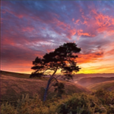
After 1000 training rounds, the network is capable of reconstructing the sunset image. However, it is still a bit blurry and contains some noticeable artefacts. The network is further trained for 2000 more rounds, after which it can produce a near perfect reconstruction of the original image.
In[]:=
trainedDec[latent]
Out[]=

Compressing 10 images
Compressing 10 images
The image reconstruction produced by the network after training with just 1 image should not be surprising because it has more than sufficient parameters to learn the image and reliably reconstruct it. The real challenge arises when it needs to learn to reconstruct multiple images. Therefore, to put more pressure on the network, it is trained with 10 images.
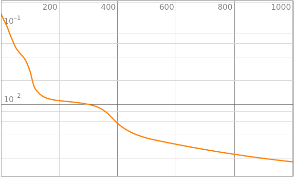
The loss curve shows an interesting pattern: The network does not learn until 600 iterations after which it suddenly starts to learn rapidly. I could reproduce this effect 3 times. Training the network with 10 input images for 3000 rounds took close to 75 minutes on an M1 MacBook Air with 8 GB RAM.
Compressing 100 images
Compressing 100 images
Training 1 image for 3000 rounds took about 6 to 7 minutes. Training 10 images for 3000 rounds increased the time to about 75 minutes. Scaling this linearly to 100 images, it would have taken about 750 minutes or 12 - 13 hours. It was thus impractical to continue further training on Wolfram since it does not support training with GPU. I ported the network to PyTorch and was able to train the network with 100 images for 5000 rounds in just about 3 hours. Further, I trained the same model with GoogleColab with a T4 instance and it completed 5000 rounds in 1 hour 20 minutes.
Results
Results
Single image trained for 1000 & 3000 rounds
Single image trained for 1000 & 3000 rounds
For the first iteration where the network was trained with only 1 example, after 3000 training rounds it was capable of a near perfect reconstruction of the original image. The left image is the original image, center is reconstruction after 1000 training rounds and the right one is the reconstruction after 3000 training rounds.
After 3000 training rounds, the error between the original image and the reconstructed image is 0.07 %, which is not bad, considering that it can be reconstructed from a mere length 30 vector.
10 images trained for 3000 rounds
10 images trained for 3000 rounds
When the network is trained for 10 images, after 3000 training rounds, there is still noticeable noise in the reconstructed images. The top two rows show the original images and the last two rows are the images reconstructed using their latent vectors.
The reconstruction is lossy and shows a film grain effect. If the network is trained for more iterations, the film grain may reduce further.
100 images trained for 5000 rounds
100 images trained for 5000 rounds
The following output is from training the network with 100 images for 5000 iterations. The top 4 images are the original ones and the ones below them are their reconstructions:
With 100 images and 5000 iterations, the outputs have the same film grain as in the case of 10 images with 3000 iterations. This strongly indicates that training for more rounds reduces the film grain.
Discussions
Discussions
Compression Ratio
Compression Ratio
A 3 x 512 x 512 image takes 786,432 bytes or 768 kilobytes. The average size of the JPEG images used for training is 40 kilobytes. This gives a compression ratio of around 20.
The neural network designed in this article compresses all images down to length 30 vectors of 32 bit float data type which is always 120 bytes when packed and serialized. This gives a compression ratio of 6553.
Of course this is not a fair comparison because the latter still depends on the neural network for the reconstruction. Additionally, the training is expensive in terms of time taken and GPU requirements.
Scaling
Scaling
There are two possible ways to make the network learn more images. The first is to train it for more rounds. As mentioned earlier, as we want the network to reconstruct the image as close as possible to the original ones, we let it to over fit as much as possible, and therefore there is no upper bound on the maximum training rounds as long as the error continues to decrease. If the error no longer reduces, then the network can no longer learn. Secondly, the network demonstrated in this article is a very shallow one. Deeper networks can learn more complex patterns and can thus learn to fit more images.
Applications
Applications
Although secondary storage is generally cheap, much of it is consumed in archiving old data. In the span of 10 -15 years, everyone has digital galleries filled with at least a 100,000 photos. Using this method presented, neural networks can be used to pack the photos down to their latent representations, saving enormous amounts of storage.
For example, my photos dating over past 10 years amount to about 120,000 and take up around 400 GB of storage. They are a mix of JPEG and HEIC formats. If I create a sufficiently deep neural network and allow it train for a week or two, I could then convert all the images into latent representations. Assuming a latent vector of length 30, for 120,000 images, the storage memory required goes down to less than 20 MB. The network itself would be at most 4 to 8 GB.
Another application that I can imagine, although a bit far-fetched, is transmission of latent vectors in low bandwidth communications, such as LoRA-WAN, which has an average data-rate of just around 300 bytes per second under poor conditions. When setup correctly, the latents could be transmitted from a source and the images can be reconstructed at a destination.
Limitations
Limitations
It remains unclear what the maximum number of images is, that a network can learn to reconstruct before it fails. The only way is to keep training with more and more images until the error no longer decreases. There is no deterministic way to estimate this.
Conclusions
Conclusions
1
.Overfitted Neural Networks can potentially be used to highly compress images into small latent representations. These latent representations can be used to reconstruct the a near perfect version of the image.
2
.When more images are required to be fit into the model, the number of training rounds should be increased.
3
.Alternatively, if the network is sufficiently deep and has enough parameters, it could learn to memorize and reconstruct large number of images.
References
References
◼
The original inspiration is taken from the work https://research.google/blog/image-compression-with-neural-networks/ in which the compression is done using recurrent neural networks instead of Autoencoder.
◼
The convolutional autoencoder design is based on the one from Aurélien Géron’s Hands-On Machine Learning book, Chapter 17: https://github.com/ageron/handson-ml3/blob/main/17_autoencoders_gans_and_diffusion_models.ipynb
CITE THIS NOTEBOOK
CITE THIS NOTEBOOK
Latent vectors as compressed images using neural network
by Soumya Sambeet Mohapatra
Wolfram Community, STAFF PICKS, December 24, 2025
https://community.wolfram.com/groups/-/m/t/3596196
by Soumya Sambeet Mohapatra
Wolfram Community, STAFF PICKS, December 24, 2025
https://community.wolfram.com/groups/-/m/t/3596196