As I was reading an excellent paper on SARS-CoV-2 transmission mechanism, I came across a few interesting statements like this one:
Fatality rates [due to COVID19] are likely to be higher in populations older than in Hubei province (such as in Europe), and in low-income settings where critical care facilities are lacking
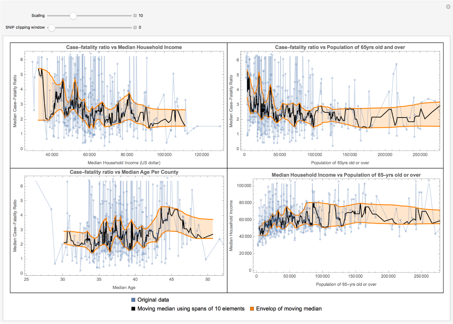
In this short essay, I’ve explored above statements computationally over US counties. My analysis suggests that the case-fatality ratio decreases by a factor of about 2 when the median household income goes from $30,000 to $60,000. However, it shows less sensitivity to incomes of $60,000 or more. Additionally, the case-fatality ratio increases slightly with the median age, as expected. On the other hand, if one considers the population of 65-yrs old and over, the case-fatality ratio shows some counterintuitive features, e.g., it decreases by this population, which is not what one expected (in fact, one may expect the reserve). The visualization of median house hold income vs population of 65yrs old and over suggests that the income increases by this population, which may imply better health care services and ultimately less fatality.
Collecting data
Collecting data
I will use NYTimesCOVID19Data function from Wolfram Function Repository to import data from the New York Times COVID-19 United States County-by-County data.
Get time series data for US counties:
In[]:=
timeseries=ResourceFunction["NYTimesCOVID19Data"]["USCountiesTimeSeries"];
I calculate the case-fatality ratio using a simple estimator from cumulative case and death values per day
Out[]//TraditionalForm=
Case-fatality ratio
Cumulative deaths
Cumulative confirmed cases
Therefore, for each day, we will have a different value for the case-fatality ratio. Additionally, I will consider days for which there has been reported deaths, and also the confirmed cases are more than 100 cases.
Drop missing keys, select counties with more than 100 confirmed cases, and generate case-fatality ratio as the ratio between cumulative value of deaths with cases per day:
In[]:=
cfr=timeseries[KeyDrop[Missing[]]][Select[#Cases["LastValue"]≥100&],<|"CaseFatalityRatio"Select[Positive][(100.#Deaths/#Cases)["Values"]]|>&][Select[#CaseFatalityRatio≠{}&]]//Normal;
Then, I will get MedianHouseholdIncome and MedianAge per county, combine it with the case-fatality ratio data and put them in one single dataset.
For each county, get MedianHouseholdIncome and MedianAge, and add it to the association:
In[]:=
ds=Apply[Join,#,{1}]&@Merge[{cfr,EntityValue[Keys@cfr,{"MedianHouseholdIncome","MedianAge"},"Association"]},Identity];
I will get the population of 65yrs old and over of US counties from census.gov website. Since this step is kind of time-consuming, I’ve iconized the data and will use it.
Get the population of 65yrs old and over per US counties from census.gov:
In[]:=
(*census=Import["https://www2.census.gov/programs-surveys/popest/tables/2010-2018/counties/asrh/PEP_2018_PEPAGESEX.zip","PEP_2018_PEPAGESEX_with_ann.csv"][[All,{3,925}]];{co,ppl65p}=Transpose@census[[3;;]]/.{"District of Columbia, District of Columbia""District of Columbia"};ppl65=AssociationThread[Interpreter["USCounty"|"USState"][co]ppl65p];*)ppl65=;
Add the population of 65yrs old and over as a new column to the data:
In[]:=
dataset=Dataset[KeyValueMap[<|"State"#1,#2,"Population65YrsAndMore"ppl65[#1]|>&][ds]];
Visualizations
Visualizations
In the following visualizations, the blue lines are the actual data, the black ones are the moving median over window of 10 elements of the actual data, and the orange ones are the envelop of the moving median (which has two parameters, σ scaling and SNIP method clipping window). Note that population data are estimated ones for 2018.
r
Plot data against the moving median using spans of 10 elements and the median envelop by preserving peaks up to scale using SNIP method:
σ
Out[]=