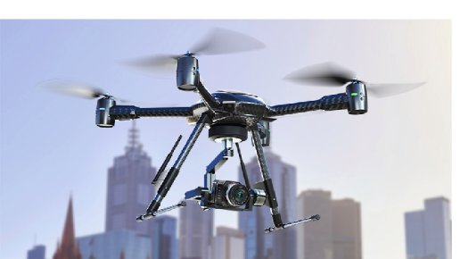
A quadcopter is a helicopter which has four equally spaced rotors, typically located at the corners of a square body. Unlike a helicopter, since quad-copters have four independent rotors, the need for a swash-plate mechanism is no longer required to increase the degrees of freedom of the system. Quadcopter helicopters present a formidable control problem due to the complexity of the system’s dynamics which have made it all but impossible to control without electronic assistance. The decrease in cost and size of microprocessors has allowed for the increased feasibility of quad-copters in the commercial, military and hobbyist domains in recent years.
Modeling the Quadcopter
Modeling the Quadcopter
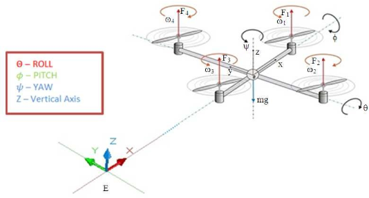
The quadcopter has three rotational and three translational degrees for freedom for a total of six degrees of freedom. Since it only has four independent inputs in the form of rotor speeds, the resulting system is severely under-actuated. Achieving the six degrees of freedom using only the four inputs would require coupling the translational and rotational motions and therefore the resulting system is highly nonlinear even without accounting for aerodynamic and gyro effects. Additionally, quad-copters are subject to negligible friction with respect to the translational motion when compared to ground vehicles and therefore require their own damping to stop and / or remain stable.
Model Legends:
Model Legends:
In[]:=
Symbol | Parameter/Variable | Value |
m r | massofdrone | 0.43kg |
ℐ x | bodygyroeffectaboutthexaxis | 0.0196 |
ℐ y | bodygyroeffectabouttheyaxis | 0.0196 |
ℐ z | bodygyroeffectaboutthezaxis | 0.0264 |
ℓ | distancetorotorfromcenterofmass | 0.25m |
g | gravitationalacceleration | 9.8m/ 2 s |
j r | propellergyroeffect | 0.01m |
u 1 | z-axistranslationalmovementinput | N |
u 2 | y-axistranslationallateralmovementinput | N |
u 3 | x-axistranslationalaftmovementinput | N |
u 4 | rotationalmovementinputaboutthez-axis | Nm |
Ω | residualangularvelocity | radians |
θ | rollangle | radians |
ϕ | pitchangle | radians |
ψ | yawangle | radians |
| positionalongthez-axis | m |
ρ | airdensity | kg 3 m |
s | effectivesurfacearea | 2 m |
c d | dragcoefficient | // |
The model parameters as a list of replacement rules:
pars={0.43`,2,1.56`,3.51`,ℓ0.1`,0.01`,Ω10,g9.8`,s0.012935458`,ρ1.225`,1.3`}
m
r
ℐ
x
ℐ
y
ℐ
z
j
r
c
d
The equations of motion in terms of the torques along the principal axes and acceleration along the vertical axis are nonlinear:
In[]:=
eqns=[t](ℓ[t]-(Ω)[t]+((-)[t])[t]),[t]+(ℓ[t]-(Ω)[t]),[t](ℓ[t]+(-)[t][t]),[t]-g+ρs+;
′′
ϕ
ℐ
x
u
2
j
r
′
θ
ℐ
y
ℐ
z
′
θ
′
ψ
′′
θ
(-+)ϕ'[t]ψ'[t]
ℐ
x
ℐ
z
ℐ
y
ℐ
x
u
3
j
r
′
θ
′′
ψ
ℐ
z
u
4
ℐ
x
ℐ
y
′
θ
′
ϕ
′′
1
2
c
d
2
'[t]
(Cos[θ[t]]Cos[ϕ[t]])[t]
u
1
m
r
The equilibrium points of the system:
In[]:=
eqns[[-1]]/.{Derivative[_][_][t]:>0,(θ|ϕ)[t]->0};{=[t]/.Solve[%,[t]][[1]]}/.pars
u
1eq
u
1
u
1
Out[]=
{4.214}
In[]:=
eqns/.[t]->/.{Derivative[_][_][t]:>0,_[t]:>0}
u
1
u
1eq
Out[]=
{True,True,True,True}
Controlling the Quadcopter
Controlling the Quadcopter
With the equations of motion, it is now possible to simulate the system. A nonlinear model of the system using the parameters previously listed can be computed using the symbol. The states of the system are the angular positions along the principal axes ϕ, θ and ψ and the corresponding angular velocities as well as the vertical position and velocity ’, for a total of eight states. The inputs of the system are the forces and torques , and the outputs are the angles and vertical position. Finally, the independent variable is specified.
u
i
t
In[]:=
drone=NonlinearStateSpaceModel,{ϕ[t],ϕ'[t],θ[t],θ'[t],ψ[t],ψ'[t],[t],'[t]},{{[t],},[t],[t],[t]},{ϕ[t],θ[t],ψ[t],[t]},t/.
u
1
u
1eq
u
2
u
3
u
4
Out[]=

ϕ[t] | x. 1 |
x. 1 | 2-0.1 x. 2 x. 2 x. 3 u 2 |
θ[t] | x. 2 |
x. 2 | 0.967949 x. 1 x. 3 x. 2 u 3 |
ψ[t] | x. 3 |
x. 3 | 3.510.44 x. 1 x. 2 u 4 |
[t] | x. 4 |
x. 4 | -9.8+0.0102999 2 x. 4 u 1 |
ϕ[t] | |
θ[t] | |
ψ[t] | |
[t] |
The open loop response can be simulated using the symbol. The drone we set the initial conditions to on all angles and meter height on the z-axis. Predictably, the drone falls freely without feedback control:
0
1
In[]:=
srol=OutputResponse[{drone,{0,0,0,0,0,0,1,0}},{0,0,0,0},{t,0,10}];Plot[%[[4]],{t,0,10},PlotRangeAll,AxesLabel{"s","m"}]
Out[]=
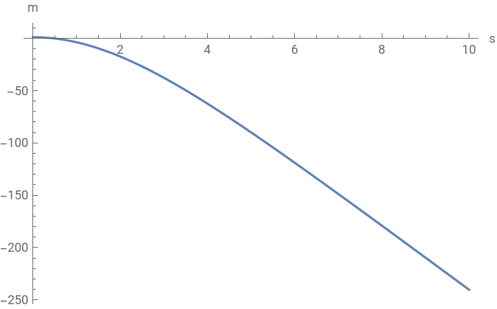
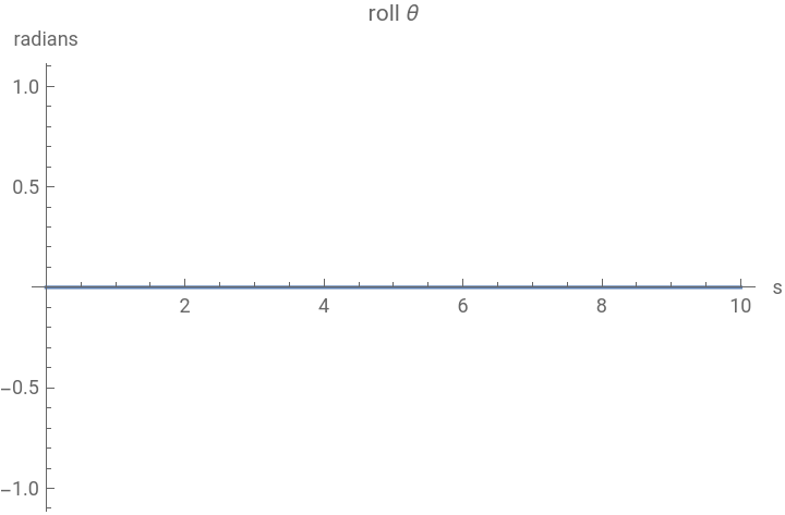
The remaining states remain constant, as the drone is modelled as a perfectly symmetrical square:
In[]:=
Plot#[[1]],{t,0,10},&/@Thread
Out[]=
,
,
Controller Design and Implementation
Controller Design and Implementation
An estimator-regulator controller is used for the control of the drone in this example. Controlling the drone’s altitude is a tracking problem. In our model the altitude corresponds to the fourth output. We can specify it as an association:
In[]:=
drone=NonlinearStateSpaceModel[drone,Automatic,Automatic,Automatic,None];sspec=<|"InputModel"->drone,"TrackedOutputs"->4|>;
The design of the optimal regulator involves choosing a set state weights , where is a semi-positive definite matrix dimensionally equal to the state matrix . Tracking an output signal increases the dimensions of by :
q
q
A
q
1
In[]:=
{,}={10DiagonalMatrix[{1,1,1,1,1,1,1,1,1}],DiagonalMatrix[{1,1,1,0.1}]};MatrixForm/@%
Out[]=
,
10 | 0 | 0 | 0 | 0 | 0 | 0 | 0 | 0 |
0 | 10 | 0 | 0 | 0 | 0 | 0 | 0 | 0 |
0 | 0 | 10 | 0 | 0 | 0 | 0 | 0 | 0 |
0 | 0 | 0 | 10 | 0 | 0 | 0 | 0 | 0 |
0 | 0 | 0 | 0 | 10 | 0 | 0 | 0 | 0 |
0 | 0 | 0 | 0 | 0 | 10 | 0 | 0 | 0 |
0 | 0 | 0 | 0 | 0 | 0 | 10 | 0 | 0 |
0 | 0 | 0 | 0 | 0 | 0 | 0 | 10 | 0 |
0 | 0 | 0 | 0 | 0 | 0 | 0 | 0 | 10 |
1. | 0. | 0. | 0. |
0. | 1. | 0. | 0. |
0. | 0. | 1. | 0. |
0. | 0. | 0. | 0.1 |
The optimal regulator (LQR) can now be computed:
The closed-loop poles of the closed-loop system with the LQR can be a useful reference to compute the estimator gains since the estimator poles must be faster than the regulator poles. We can obtain the closed-loop regulator poles from the data-object as a property:
The estimator gains can now be computed using faster poles than the closed-loop poles with the closed-loop system with the LQR in the feedback path:
With the with the estimator and regulator gains, we can now assemble the estimator regulator:
The closed-loop system with the estimator regulator in the feedback path:
While the controlled system has a satisfactory performance, it is important to asses the control effort. If the control effort requires an unreasonable amount of energy, the system is unfeasible! We can assess the control signal by measuring the controller’s signal to the plant. We start by obtaining the controller model from the controller data-object via it’s corresponding property:
Next, the inputs of the controller model which consist of the reference input, the output feedbacks and state feedbacks:
The output response of the controller model yields the control signal. We can see that the control effort for this design is reasonable, peaking at around 8 Newtons: