ABSTRACT (original article): We specialize techniques from topological data analysis to the problem of characterizing the topological complexity (as defined in the body of the paper) of a multiclass data set. As a by-product, a topological classifier is defined that uses an open subcovering of the data set. This subcovering can be used to construct a simplicial complex whose topological features (e.g., Betti numbers) provide information about the classification problem. We use these topological constructs to study the impact of topological complexity on learning in feedforward deep neural networks (DNNs). We hypothesize that topological complexity is negatively correlated with the ability of a fully connected feedforward deep neural network to learn to classify data correctly. We evaluate our topological classification algorithm on multiple constructed and open-source data sets. We also validate our hypothesis regarding the relationship between topological complexity and learning in DNN’s on multiple data sets. CITATION (original article): Griffin, Christopher and Karn, Trevor and Apple, Benjamin (2024), Topological learning in multiclass data sets, Phys. Rev. E 109, 024131. https://doi.org/10.1103/PhysRevE.109.024131
Introduction
Introduction
In a previous post and in this paper in Physical Review E, we discussed a method for analyzing multi-class data using a custom topological data analysis algorithm. We focused explicitly on understanding when learning in neural networks fails and why that might be caused by topological features in the data. A by-product of that work was a topological classifier and manifold reconstruction algorithm, which we discussed briefly but not completely. In this post, we will investigate the manifold reconstruction algorithm and show how is can be used to reconstruct not only abstract vector data but also more interesting data sets like the the MNIST. This reconstruction is discussed in the Physical Review E, but here we will provide the code and a more complete description. We’ll begin with a review of some of the topological functions in the previous post.
Before we start, if you’re downloading this notebook and the files that go with it, you should probably set your working directory to wherever you put the files.
SetDirectory["YOUR DIRECTORY HERE"];
Building a Cover for a Data Set
Building a Cover for a Data Set
Reduction Code for Skeletons
Reduction Code for Skeletons
Helper Functions for Topological Computation
Helper Functions for Topological Computation
A Simple Example
A Simple Example
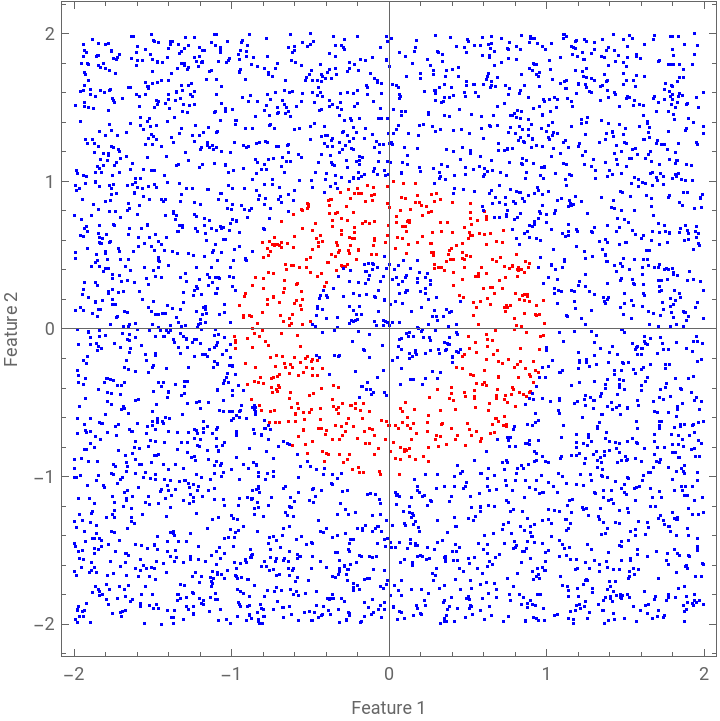
We’re going to build some data that models an annulus. Class 1 will form the annulus and Class 0 will be the data around the annulus. This is not a linearly separable data set, but it will illustrate what we’re doing. Incidentally, this is the same basic example from our earlier post, but without the Cěch complex part.
Build the Data
Build the Data
In[]:=
myNN=4000;
In[]:=
rawData=RandomReal[{-2,2},{myNN,2}];
In[]:=
classData=Map[Function[{xx},If[And[xx.{{1,0},{0,1}}.xx≤1,xx.{{1,0},{0,1}}.xx>=1/4],1,0]],rawData];
In[]:=
myClassOne=Table[If[classData[[ii]]1,rawData[[ii]],Nothing],{ii,1,myNN}];
In[]:=
myClassZero=Table[If[classData[[ii]]0,rawData[[ii]],Nothing],{ii,1,myNN}];
The raw data is shown below.
The raw data is shown below.
In[]:=
ListPlot[{myClassOne,myClassZero},PlotStyle->{Red,Blue},Frame->True,FrameLabel->{"Feature 1","Feature 2"},AspectRatio->1]
Out[]=
Build the Topology
Build the Topology
We start building the topological representation by building a skeleton. To do that, we first find the covering, then the corresponding adjacency matrix of the skeleton. Then we turn it into a Mathematica graph.
In[]:=
myRads=BuildRadii[myClassZero,myClassOne];
In[]:=
myAdjMat=BuildAdjacencyMatrix[myClassOne,myRads];
In[]:=
myGG=AdjacencyGraph[myAdjMat];
Assuming the data aren’t too spare, the graph should look something like a circle.
In[]:=
myGG
Out[]=
Graph


We don’t need all those vertices, so we’re going to find a sub-cover.
In[]:=
myComponentCover=FindComponentCover[myGG];
The red vertices are the vertices that can be used to cover the entire data set and thus can be used as a witness complex. That is a smaller simplicial complex that describes the entire data set well.
In[]:=
HighlightGraph[myGG,myComponentCover]
Out[]=
Graph
Assuming the data is dense enough, this should form an object that looks lie it has a big hole in it.
In[]:=
mySkeleton=BuildWitnessSkeleton[myClassOne,myRads,myComponentCover];
In[]:=
Show[mySkeleton,Graphics[Map[Function[{idx},Circle[myClassOne[[idx]],myRads[[idx]]]],myComponentCover]],ListPlot[myClassOne,PlotStyle->Darker[LightRed]]]
Out[]=
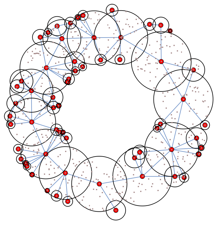
The clique simplex tends to have more holes than the Čech simplex because we’re assuming connectivity is sufficient to fill in the faces in the clique simplex. However, since we’re looking for features at the level of Class 0 (not necessarily features in Class 1) , we don’t really care.
In[]:=
myCliqueSimplex=BuildCliqueSimplex[mySkeleton,Length[First[FindClique[mySkeleton]]]];
In[]:=
ResourceFunction["BettiNumbers"][myCliqueSimplex]
Out[]=
{1,2,0,0}
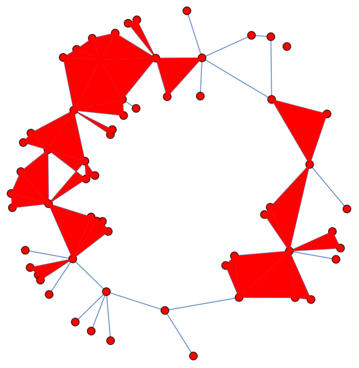
Drawing the cover with cliques filled in illustrates the Betti numbers. Holes may be visual artifacts. Each hole has to be inside a polyhedron with clear vertex points.
In[]:=
DrawWitnessComplex[myClassOne,myComponentCover,mySkeleton]
Out[]=
Joint Class Graph
Joint Class Graph
MNIST
MNIST
Now let’s do some image analysis. Let’s start by getting some MNIST data from the Wolfram Repository.
In[]:=
trainingData=ResourceData["MNIST","TrainingData"];
In[]:=
testingData=ResourceData["MNIST","TestData"];
We’ll sort the images into a table corresponding to the class. These will be our inputs.
In[]:=
theImages=Table[Map[Function[{row},If[row[[2]]==ii,row[[1]],Nothing]],trainingData],{ii,0,9}];
The following code will build a complete topological covering of the MNIST classes. Notice we’re passing in the ImageDistance function. It takes a little while to run (on an i9 or M1) so below we’ve got the data preloaded from an *.mx file. That file is provided with this post. Running time, by the way, is the real challenge with all these topological methods. They are doing non-linear manifold reconstruction, no matter how you slice it.
Let’s load the results.
One way to tell how complex the boundary structure is in the data is to see what percent of each class is needed to form a cover and whether the simplicial complex is connected (has 0th Betti number equal to 1).
Those percentages are pretty small. It looks like 0 and 1 both separate well as does 6 (for some reason). The others require more of the training set to reconstruct the manifolds. We can use the radii information to take a cross section of the data. Images with large radii are extremely far from the boundary and “should” represent more archetypical digits.
Let’s extract the images with radii in the 99th percentile. These should look like the numbers they represent. (And they do.)
Now let’s find the numbers closest to the boundaries. Those are the ones with the smallest radii, so in the first percentile.
It’s easy to see why these are boundary cases. In fact, that one “3” looks an awful lot like a “9”. It might even be an error in the data set. This is a topological way to analyze the data, even if you can’t compute Betti numbers -- which on this data set is a little hard on a laptop.
If you’ve read the Physical Review paper or the ArXiv paper that corresponds to it, you might notice these are slightly different from what’s in the paper. This may be due to code tweaks from what’s in the SI (and in one case a bug fix) or versions of Mathematica.
Visualizing the Manifolds
Visualizing the Manifolds
Now let’s visualize the manifold. We’ll have to build the graph components first. This takes a little time. I’ve save everything to a *.mx file that you can load to avoid running the process. Remember, we are doing a lot of comparisons in building these graphs.
Now we can actually build a graph. This is the thing that we’d pass into the GraphEmbedding function in order to draw a nice picture. Depending on how you build the graph, it can take a lot of time or a little time. You can pre-load the graph or build your own by uncommenting the code below. You may get a different picture, the dropout routine is randomized.
Here we can (optionally) import the graph that was saved. It can take a little while to import.
Now we’ll draw the joint graph representing all the manifolds, suppressing the edges. This graph is really a skeleton of a simplicial complex.
You’ll notice this looks a little different from the figure in the Physical Review paper or the figure on ArXiv. There’s two reasons. First, this is a randomized algorithm. But second, there was a small typo in my code when I generated the image that got published (I believe it’s still in the SI). The corrected code is in this post.
Using the Manifold Reconstruction for Classification
Using the Manifold Reconstruction for Classification
Now let’s use the manifolds we’ve reconstructed to do classification. This won’t work quite as well as LeNet but it does work surprisingly well. Below is the topological classification algorithm. It’s fairly straightforward. Using the topological covering we just compare a test point to the elements of the covering in each class. The closest point (or points) wins. It’s essentially k-nearest neighbors but with the cover sets replacing the points. In this case, you’re using a point-to-set distance, so if you’re inside one of the covering sets, the distance is zero. The interesting thing about this is you can determine if a point will cause confusion by being in multiple covering sets from multiple classes. This is a test point near the boundary. The algorithm implements a simple tie-breaking rule.
The code below will run through the test images and try to classify them. Unlike a neural network, this is a little slow. (There are many ways to improve the running time of these algorithms, but the goal is not to make a better classifier -- we have a lot of them -- it’s to study the geometrical properties of the data set as it pertains to learning.)
Below we use a confusion matrix to see how well the topological reconstruction works as a classifier. It works surprisingly well.
Comparison to LeNet
Comparison to LeNet
To see how surprisingly well, the topological method works, we can compare its output to LeNet.
Notice the neural networks run much faster than the topological reconstruction.
Obviously LeNet outperforms the topological analysis in both speed and accuracy. (It would be insane if it didn’t.) But the important take away is not neural networks do better. It’s that they don’t do better by much. Certainly a 3% accuracy improvement is nothing insignificant, but it suggests that the performance gains of LeNet (or any CNN) over basic manifold reconstruction must be coming either from generalization or from managing boundary points. Using the topological reconstruction, we can check that.
Below is a little function that takes test results and produces a summary of their characteristics.
Here is another function that will render the results nicely with the TableForm command. This returns two tables a global summar
We can run these commands on the whole MNIST data set as follow:
We see that 86.8% of the test data is actually “in sample”. That means that the power of LeNet (and the topology model is dealing with a small number of off-manifold points and boundary points. These are samples that are in at least two covering elements in two different classes. We can zoom in a little more.
The biggest errors come from misclassification of boundary points and incorrect generalization. Points that are “in manifold” and incorrect are in the reconstructed manifold of the wrong class. This is also a generalization problem. We could zoom into specific classes, if needed, but the point is. LeNet’s power seems to be a little bit of generalization and boundary resolution, since only 5% of the test data is actually outside the sample, when the manifolds in question are reconstructed using Wolfram’s ImageDistance metric.
Conclusion
Conclusion
In this notebook, we’ve constructed some general algorithms to reconstructing manifolds using topological data analysis and then used those reconstructions to analyze the performance of a neural network. This work is interesting because everything comes down to the metric you choose on the data set. (If you re-did all this with a Euclidean metric, you get much worse performance on the classification.) In particular if you have data in classes and you can define a metric, then you can use these techniques on your data.
The main drawbacks to manifold reconstruction (and some forms of topological data analysis) is performance. The proposed methods can be parallelized, but in the end the algorithm is still quadratic and there is still the issue of the No Free Lunch theorem, which suggests this can’t really be sped up arbitrarily unless P = NP. What you gain from the extra time spent is a tool for analyzing a data set, especially with respect to its use in neural network training and testing.
There are definitely some areas of future work. Obviously speed up is a huge issue and that comes into play when dealing with things like finding higher order Betti numbers for large manifold reconstructions (big simplicial complexes or graphs). Additionally it would be nice to be able to run this on a data set without classes, which you can do by artificially clustering your data (using FindClusters) and then running these algorithms, but that’s an area of future study.
CITE THIS NOTEBOOK
CITE THIS NOTEBOOK
Analyzing and visualizing multi-class data sets using topological data analysis
by Christopher Griffin, Trevor Karn & Benjamin Apple
Wolfram Community, STAFF PICKS, June 6, 2025
https://community.wolfram.com/groups/-/m/t/3475710
by Christopher Griffin, Trevor Karn & Benjamin Apple
Wolfram Community, STAFF PICKS, June 6, 2025
https://community.wolfram.com/groups/-/m/t/3475710