A integral part of the WPP is that non-deterministic computations in the form of rewriting systems can produce emergent geometries. This project more thoroughly studies how these geometries can form from rules of certain length and specific rewrite conditions by looking at some combinations of length 1 and length 2 rules. It also delves into what it is in these rewrite systems that allow higher dimensions, and what a spatial dimension may be thought of from a more abstract and discrete level. The goal of this project is to gain a better understanding of what rules may be capable of leading to certain geometries and why they affect the initial conditions in such a way.
◼
A Brief Introduction to Quivers and Rewrite Systems
A Brief Introduction to Quivers and Rewrite Systems
For a more in depth introduction to these topics, visit https://quivergeometry.net/graphs-and-quivers/ and https://quivergeometry.net/rewriting-systems/.
In this project we’ll be looking at quivers and rewrite systems, but what are those? A cardinal quiver is can be thought of as a type of directed graph - each edge is labeled with what we call a cardinal. Cardinals must be locally unique; a cardinal can not enter (or leave) the same vertex twice. This allows for an unambiguous sense of direction. Below we have a simple line quiver. The red arrow is the cardinal, and it points in the direction of the edge. The below quiver would start at the left point and travel across the cardinal to the right.

GQGLineQuiver[2]
Out[]=

These quivers will be describing rewrite systems - systems that change over time. We begin by applying a well defined rule to a structure. In the case of this project, we’ll be using ordered strings. The rule picks out a chosen sub-element from the given string and transforms it into something else. We then take the changed string and repeat the process with the same rule, rewriting the string over again until the rule can’t be performed anymore. This project aimed to take a binary string of finite length and study how geometry can emerge over rules of different lengths. In this project I studied length 1 and length 2 rules on finite strings using the unique characters ■ and □, which one can also think of as the binary numbers 1 and 0 respectively.
Emergent Geometry from Quivers
Emergent Geometry from Quivers
Before we begin we must first understand how geometry can emerge through directed graphs.
Let’s say you have an ordered pair {x,y} where x and y are any integer. For our initial condition let’s let x=0 and y=0.
Let’s say you have an ordered pair {x,y} where x and y are any integer. For our initial condition let’s let x=0 and y=0.
In[]:=
$sq5=SquareQuiver[5,ImageSize->"ShortestEdge"->50, VertexLabels->"Name", ArrowheadSize->16,EdgeThickness->3,VertexSize->7, GraphOrigin->TupleForm[0,0]];TupleForm[args___]:=Row[{"(",Row[{args},","],")"}]$sq5=MapVertices[Function[TupleForm@@((List@@#)-3)],$sq5];ExtendedGraph[$sq5,ViewRegion->{Path[GraphOrigin,""]}]

Next, let’s define an operator y. All y does is act on an initial condition and change it’s y-coordinate by 1. If you applied y to the list {0,0}, you would add 1 to the second element in the ordered pair and get {0,1}. We can graph this change using a cardinal that represents the application of y, with the tail of y being the initial condition and the head of y connecting to the result of y’s action on {0,0}, which in this case is {0,1}.
In[]:=
ExtendedGraph[$sq5,ViewRegion->{Path[GraphOrigin,"y"]},GraphLegend->
"y - (0, +1)"]

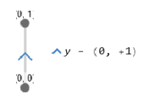
You can think of the quiver y as the application of the operator y. You have an initial condition, apply y, and get a changed version of the initial condition.
Now let’s add in a second operator, called x. x does the same thing as y, but it acts on the ordered pair’s first element x instead of its second, increasing it by 1.
Now let’s add in a second operator, called x. x does the same thing as y, but it acts on the ordered pair’s first element x instead of its second, increasing it by 1.
ExtendedGraph[$sq5,ViewRegion->{Path[GraphOrigin,"x"]},GraphLegend->
"x - (+1, 0)"]

Out[]=
x - (+1, 0) |
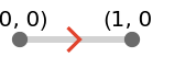
After applying x to our initial condition, we can apply x again or apply y.
ExtendedGraph[$sq5,ViewRegion->{Path[GraphOrigin,"xy"],Path[GraphOrigin,"xx"]},GraphLegend->{
"y - (0, +1)",
"x - (+1, 0)"}]
Out[]=
|
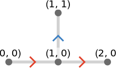
We can also add our y operator acting on our initial condition back in. Now our IC, (0,0), takes the x operator to (1,0). From there it has two choices. It can take the y operator to (1,1) or the x operator once more to (2,0). You can repeat this process with these new initial conditions to obtain an infinite grid.
$infSq=SquareQuiver[7,PeripheralVertices->Automatic,GraphLegend->{
"y - (0, +1)",
"x - (+1, 0)"},ImageSize->"ShortestEdge"->50, VertexLabels->"Name", ArrowheadSize->16,EdgeThickness->3,VertexSize->7,GraphOrigin->TupleForm[0,0]];$infSq=MapVertices[Function[TupleForm@@((List@@#)-4)],$infSq]
Out[]=
|
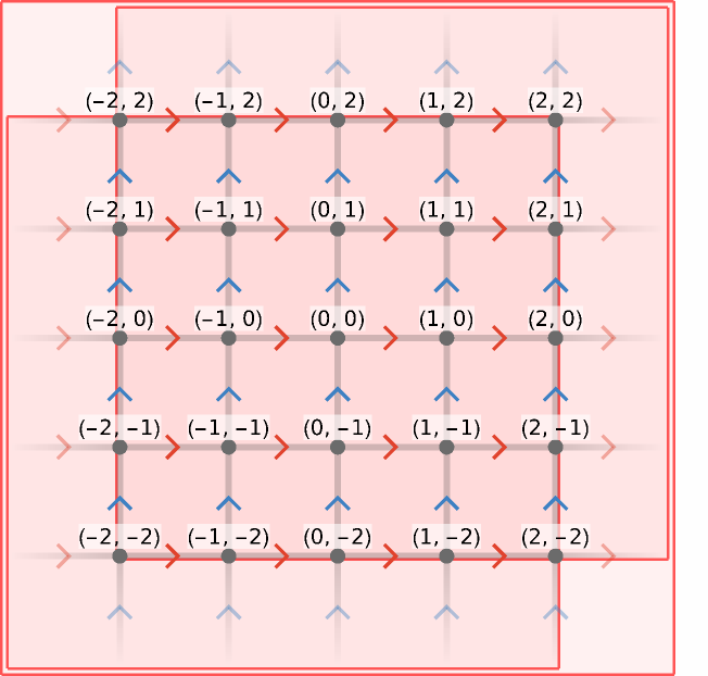
All we’ve done here is show all possible outputs for a given initial condition, with no restraint on how many times an operator can be applied. But out of that we made an object that looks just like the Cartesian plane! We could also add a third element to the ordered pair {x,y} to make an ordered triple {x,y,z} and a third operator named z that increases the third element of the list by 1. Through the same process we went through here, we could then make an object that is isomorphic to . Generally speaking, you can make an object isomorphic to by repeating this process with a list of n elements.
3
n
Length 1 Rules
Length 1 Rules
First, we have the “Trivial” length 1 rules. These change nothing in the initial condition (referred to as IC), so they only create self-loops within the IC’s multiway quiver.
GQGruleGalleryForm[a_]:=SpacedColumn[RewriteForm@@@a,Spacings->20];Row[{"The trivial length 1 rules:",ruleGalleryForm[{"■"->"■","□"->"□"}]}]
Out[]=
The trivial length 1 rules:
■■ |
□□ |
Clear[niceStringRewritePlot];niceStringRewritePlot[rule_,rules___Rule][ic_]:=niceStringRewritePlot[rule,ic,rules];niceStringRewritePlot[rule_,ic_String,opts___]:=RewriteQuiver[ toSRSystem[rule],ic,opts, ArrowheadPosition->0.4,VertexShapeFunction->"Vertex"->StringPlot, EdgeColorFunction->"Cardinal",ImagePadding->15, ImageSize->"ShortestEdge"->40,VertexLayout->TreeVertexLayout[Orientation->Top]];toSRSystem[rule_Rule]:=StringRewritingSystem[rule];toSRSystem["Circular"->rule_Rule]:=CircularStringRewritingSystem[rule];niceStringRewritePlot["■"->"■","■□■"]
Out[]=
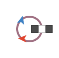
Obviously, the loop will have k cardinals for k black cells. Nothing else will change with string length or addition of other unique characters. The same applies with it’s inverse, □□ - k cardinals for k white cells.
Next are the length 1 “Conversion” rules:
Row[{"The length 1 conversion rules:",ruleGalleryForm[{"■"->"□","□"->"■"}]}]
Out[]=
The length 1 conversion rules:
■□ |
□■ |
These simply shift black to white or white to black. One may also think of it as turning a bit ‘off’ ( ) or ‘on’ () .
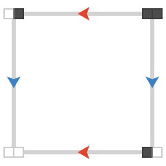
Below, you’ll see the rule applied to a finite number of black cells (■) from k=1 to k=4, with k being the number of black cells in the IC. A pattern quickly forms, graphing a k-dimensional hypercube on the multiway quiver with an initial condition of k black cells.
■->□=1->0
□->■=0->1
Below, you’ll see the rule
■->□
characterMaskVector[pos_][str_]:=Part[Characters@str,pos]/.{"1"->1,"0"->0};consumptionQuiver[init_,showLabel_:True,opts___Rule]:=RewriteQuiver[StringRewritingSystem["1"->"0"],init,opts,ImageSize->"ShortestEdge"->If[showLabel,100,75],ImagePadding->5,VertexCoordinateFunction->characterMaskVector[FirstColumn@StringPosition[init,"1"]],ArrowheadShape->"Cone",EdgeThickness->3,ViewOptions->{SphericalRegion->True,ViewProjection->"Orthographic"},VertexShapeFunction->If[showLabel,"Vertex"->StringPlot,"Point"],VertexOverlapResolution->1];consumptionList={consumptionQuiver["1"],consumptionQuiver["11"],consumptionQuiver["111"],consumptionQuiver["1111"]};SpacedRow[{"k=1","k=2","k=3","k=4"}->consumptionList]
Out[]=
 |  | ||
k=1 | k=2 | k=3 | k=4 |

Cubes from Length 1 Conversion rules
Cubes from Length 1 Conversion rules
Why is it that the conversion rules form a k-dimensional hypercube? Instead of acting on a list of integers, we’re acting on a string of finite size with a finite number of states. Instead of being able to increase an integer forever, there are only so many options available to us. The conversion rule ■->□ will take any black cell and turn it white, so with k black cells, you will always end up with an all white cell block after k runs of the rule. So, we have a run of black cells and a run of white cells. Now we just need to figure out how to get there.
■■■ will always turn into □□□ after 3 rewrites with the stated rule, but there’s no single way to get there. For the first rewrite, we could take any of the 3 blocks and turn them white. From that rewrite we have 2 blocks which we could turn white, and from there only 1. But we can turn these blocks in any order. We could choose to turn the second block white first, and then the third, and then the first, or any other combination of the three.
■■■ will always turn into □□□ after 3 rewrites with the stated rule, but there’s no single way to get there. For the first rewrite, we could take any of the 3 blocks and turn them white. From that rewrite we have 2 blocks which we could turn white, and from there only 1. But we can turn these blocks in any order. We could choose to turn the second block white first, and then the third, and then the first, or any other combination of the three.
At one rewrite, all possible strings will be one row down from the initial condition, and so on. But there’s also something interesting going on. Because the string is ordered, there are actually three different ‘sub’ operations that can be done to it. The red quiver acts only on the first element of the string, the blue acts only on the second, and the green will only act on the third.
Length 2 Rules
Length 2 Rules
Next I started to look at all the length 2 rules. There’s 16 of them, and I was able to sort them into four types. First, there are the ‘trivial’ types. Like the length 1 trivial rules, these don’t change anything about the IC. The rewrite quiver is just a self loop.
Next we have the length 2 ‘conversion’ rules. These work exactly like the length 1 rules we just looked at when there’s an even amount of black cells, but some small differences appear due to a finite number of black cells and the fact that follows - there may not always be a way to fully convert the string to white.
I wasn’t able to find any interesting geometry that came out of these cases.
Cuboids from Length 2 Gobbling Rules
Cuboids from Length 2 Gobbling Rules
The last thing I studied were the length 2 ‘gobbling’ rules, called this because they would take a cell to the left or right and ‘eat’ them up. Here they are:
Each time the rule is applied to the IC, a quiver corresponding to the coordinate it affects is taken, and the cell turns black. This repeats until the entire string is black.
However, if we were to add in a second black cell, let’s say at the fourth element, we’d then have two quivers that could be taken.
However, if we were to add in a second black cell, let’s say at the fourth element, we’d then have two quivers that could be taken.
From that point we’d have two more quivers branching off from those new initial conditions, and just like in our length 1 conversion rules, this process will repeat until there are no black cells left in either ‘run’ of white cells.
Generally speaking, if you have two runs of white cells of length m and n, the resulting rectangle will be mxn. By adding a third or fourth run of a single black cell followed by white, you can extend the cuboid into other dimensions.
Concluding Remarks and Future Plans
Concluding Remarks and Future Plans
The underlying thesis of the WPP is that non-deterministic computations in the form of rewriting systems can produce emergent geometries. Looking at the simplest string rewriting systems we can devise nice coordinate systems that make the underlying geometry simple, and explain it in terms of familiar quivers and their cardinal structure. This can be done for gobbling and length 1 conversions, which respectively create objects isomorphic to cubes and cuboids. However it remains future work to define coordinate systems for the remaining rules in these simple families. For example, I didn’t have enough time to finish studying the length 2 rules, but I hope to do so in the near future. The rules that I didn’t study are listed below:
The length 2 sorting rules yielded some interesting geometrical results, and the replacement rules resembled lattices. I was able to figure out exactly how each rewrite rule covered would function given a certain initial condition, but I have yet to figure a pattern out for the above sorting and replacement rules. I also have yet to explore circular rewrite systems and systems with more than two characters, both of which can yield some interesting symmetrical results.
Acknowledgements
Acknowledgements
Massive thanks to my mentor, Taliesin Beynon, for guiding me through this project and helping me through the Wolfram Winter School. I couldn’t have done any of this without you. Your advice, ideas, code snippets, quiver repository, and willingness to meet with me no matter the time of day has really made my experience at the Winter School worth it. Thank you to everyone else in the Winter School as well, specifically Xerxes Arsiwalla and Stephen Wolfram. I wouldn’t have gotten here without you two leading and teaching the WWP every step of the way.