Xenobots are synthetic lifeforms that are automatically designed by computers to perform some desired function and they are put together by combining different biological tissues. They are produced with the help of evolutionary algorithms - which takes in two building blocks along with a behavioral goal. Using 2D cellular automata as a model for Xenobots, this essay aims to produce a genetic algorithm that will find growth rules to produce a population that meets a certain criteria.
Introduction
Introduction
Genetic algorithms are based on the concept of natural selection where the fittest individuals in a certain population are selected to reproduce offspring which form the next generation. In this essay, the algorithm is initialized with a population of 50 randomly configured cellular automata. This population is first doubled - mutated copies of each automata in the original population are created. This process provides variations. Next, a new generation of 50 cellular automata is chosen from the current generation through the selection process, which is based on the fitness function. The fitness function being used in this essay is a measure of the difference between the shape of the 2D cellular automata and a square - the end objective is to have a population where every cellular automata is as close as possible to a square.
Genetic Algorithm
Genetic Algorithm
2D Cellular Automata
2D Cellular Automata
Cellular Automata are examples of programs define by basic rules. A 2D cellular Automata consists of a grid of black or white cells that are updated in a series of steps according to definite rules that involve the 8 immediate neighbours of any given cell.
Progression of a 2D Cellular Automata starting from a single cell initial condition
exampleCA = CellularAutomaton[<|"Dimension" 2, "GrowthCases" {1,7}|>, {{{1}},0}, 10];ListAnimate[ArrayPlot[#, Mesh True]&/@exampleCA]
Out[]=
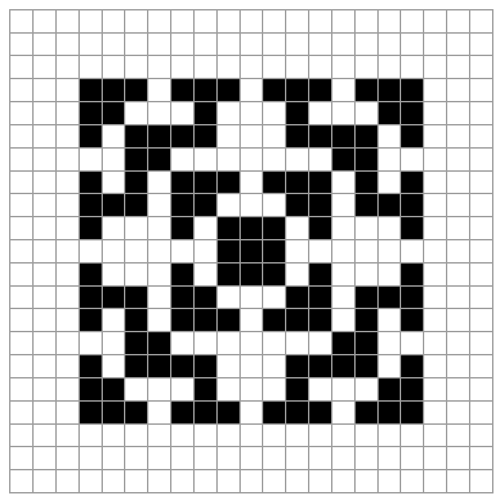
3 Dimensional Progression of the same 2D cellular Automata (shows every new generation in addition the previous generations)
ListAnimate[ArrayPlot3D[exampleCA[[1;;#]]]&/@Range[Length[exampleCA]]]
Out[]=

Defining Functions
Defining Functions
Growth cases can be used as the rule condition for cellular automata. With , a cell goes from value to value if it has neighbors that are ; otherwise it stays the same as before. This works the same way for 2D cellular automata - every cell can have 8 possible neighbours. The dimensions are also defined by saying
"GrowthCases"->{,,…}
g
1
g
2
0
1
g
i
1
"Dimension"2.
Defining a function to produce a 2D cellular automata given a certain growth case
In[]:=
producingCA[growthcase_]:= CellularAutomaton[<|"Dimension" 2, "GrowthCases" growthcase|>, {{{1}},0}, 5];
The mutations are done to the list of growth cases used to make a given generation of cellular automata. Essentially a random spot in the growth case is chosen, and the number at the random spot is replaced with another random number. The function outputs a mutated list of growth cases that can be used to produce a population of cellular automata.
Defining a mutation function that mutates a list of growth cases for cellular Automata
In[]:=
mutationFunction[growthcases_]:=Map[ DeleteDuplicates[ReplacePart[#,RandomChoice[Range[1,Length[#],1]] RandomChoice[Range[0,8,1]]]]&, growthcases]
In this particular essay, our end goal is to get our cellular automata as close as possible to the shape of square. Using growth cases over 5 iterations of 2D cellular automata produces a final output of either a 1x1 grid, 3x3 grid or 11x11 grid. Using lists of possible configurations in these grids, the least difference between the current shape of the cellular automata and a possible square shape is calculated. This is then divided by the total number of cells and this ratio is chosen as the value for the fitness function. It is also important to note that 1x1 2D cellular automata are not suitable for our purpose and they are therefore given the maximum fitness of 1.
The configurations are as follows:
For a 3x3 grid of cells: A single black square in the middle
For a 11x11 grid of cells: A 5x5 square of black cells at different locations in the 11x11 grid.
For a 3x3 grid of cells: A single black square in the middle
For a 11x11 grid of cells: A 5x5 square of black cells at different locations in the 11x11 grid.
Defining the fitness function
In[]:=
list1=;list3=;list11= ;calculatingDiff[CAStep_,triangle_]:=(Module[{counters=0},Do[Do[If[CAStep[[i]][[j]]≠ triangle[[i]][[j]], counters=counters+1, counters=counters], {i, Length[CAStep]}], {j,Length[CAStep]}];Return[counters]];)fitnessFunction[finalOutputOfCA_]:=Divide[Min[calculatingDiff[finalOutputOfCA, #]&/@(Which[Length[finalOutputOfCA]1, list1, Length[finalOutputOfCA]3, list3, Length[finalOutputOfCA]11, list11])],Length[finalOutputOfCA]*Length[finalOutputOfCA]];
The new generation is produced by adding a mutated population which is produced by the mutated growth cases to the original parent population.
Creating a new generation of cellular automata
In[]:=
producingGen[parentGen_, mutatedGC_]:=Join[parentGen, Map[producingCA,mutatedGC]];
Two parameters need to be passed on the new iteration of the algorithm - both the 50 fittest cellular automata and the 50 growth rules that produce these 50 fittest cellular automata. This is why two selection functions are used. Fitness for every member in a generation is calculated and the ones which give the least value for fitness are chosen.
Defining selection function that chooses the fittest cellular automata
selectingCA[ListCA_]:=Join[Keys[Sort[AssociationThread[ListCA,Length[fitnessFunction[ListCA[[#]][[-1]]]&/@Range[Length[ListCA]]]]]],ListCA][[;;50]]
Defining selection function that chooses the growth rules that correspond with this fitter population
In[]:=
selectingGC[CombinedListGC_, ListCA_]:=Keys[Sort[AssociationThread[CombinedListGC, fitnessFunction[ListCA[[#]][[-1]]]&/@Range[Length[ListCA]]]][[;;50]]]
Updating Generations
Updating Generations
Each iteration of the genetic algorithm first creates a mutated list of growth rules (given the current list of growth rules being used). It then produces a new generation of cellular automata using these mutated growth rules. Then the fittest populations of both cellular automata and growth cases are chosen and the total fitness of this new population is calculated and appended to a list. The current list of growth rules is equated to the new list of growth rules and the current population of cellular automata is equated to the newly produced population of cellular automata.
Defining a function that runs the genetic algorithm one time
In[]:=
eachRun[] := Module[{newGenCA, newListGC, mutatedListGC, temp},mutatedListGC =mutationFunction[currentListGC];temp=producingGen[currentPopCA, mutatedListGC];newGenCA = selectingCA[temp];newListGC = selectingGC[Join[currentListGC, mutatedListGC], temp];AppendTo[listOfFitness, Total[fitnessFunction[newGenCA[[#]][[-1]]]&/@Range[Length[newGenCA]]]];currentListGC=newListGC;currentPopCA=newGenCA;]
Initialisation
Initialisation
Some variables are initialized and a population of 50 randomly generated cellular automata is created.
In[]:=
popSize = 50;initialListGC= Table[DeleteDuplicates[Table[Random[Integer, {0,8}], 9]], popSize];initialPopCA=Map[producingCA, initialListGC];
In[]:=
currentListGC = initialListGC;currentPopCA = initialPopCA;listOfFitness = {};
Running and Visualisations
Running and Visualisations
Running the genetic algorithm 25 times
Plotting the total fitness of a generation over each run of the algorithm. Since the fitness is a measure of how far away the cellular automata is from a square like shape, the lower the fitness, the better.
Here we try to visualise the initial population and compare it to the final population produced by the genetic algorithm. As can be visually observed, the newer population is closer to providing square like shapes than the initial.
Cellular Automaton closest to fitness function
Conclusion and Extensions
Conclusion and Extensions
In conclusion, the genetic algorithm structure can be effectively used to evolve populations that meet a certain criteria - in this case evolving a population of 2D cellular automata to produce the shape of a square.
Since this model is used as a representation for Xenobots, a lot alterations can be made to the fitness function to make it more suitable for that purpose. Instead of merely looking at shapes, one can create a fitness function that produces certain structures that are suitable for the various purposes of Xenobots - locomotion, swimming etc.
An addition that can be made to this algorithm is using varying number of steps to produce the 2D cellular automata. Currently this algorithm is growing a cellular automata over 5 steps but this number can be changed to give a better value for the fitness function.
References
References
Kriegman, S., Blackiston, D., Levin, M., & Bongard, J. (2020). A scalable pipeline for designing reconfigurable organisms. Proceedings of the National Academy of Sciences, 117(4), 1853–1859. https://doi.org/10.1073/pnas.1910837117