I have made previous posts trying to model the Treasury yield curve parametrically (see [1], [2], [3]). The hope was that the parameters could be used to track and possibly predict how the yield curve would evolve from its inverted state to a more normal shape. The yield curve began to change dramatically in September, but the parameters of the models did not offer any insight as to how the the yield curve was evolving. This notebook takes a different approach, fitting the data to a tenth order Chebyshev polynomial approximation. The polynomial coefficients provide little insight into the shape, but the ability to take smooth first and second derivatives does offer way to track the shape evolution. The lower order Chebyshev polynomials of the fits also provide insight as to the evolution of the curves. The approximations are derived from a monotonic interpolation, from the Wolfram Resource Function Repository. The package, ChebyshevAlgorithms is attached as a supplement.
Data and fitting
Data and fitting
In[]:=
Needs["ChebyshevAlgorithms`"]
Treasury Data
Take only first ten years of terms from Treasury data and add appropriate fed funds rate for a zero point.
In[]:=
crvs=Join[{{0,5.33}},Take[#["yieldCurve"],{2,-3}]]&/@recweek;
The built-in Mathematica function, Interpolation[], is shown with the first four interpolation orders for the recent data. While the fits are pretty good for the second and third orders, they are still wavy. Higher orders make things worse.
In[]:=
stdIFn=Interpolation[crvs[[1]],InterpolationOrder->#]&/@{1,2,3,4};ShowPlotEvaluate[#[t]&/@stdIFn],{t,0,10},,ListPlotcrvs[[1]],
Out[]=
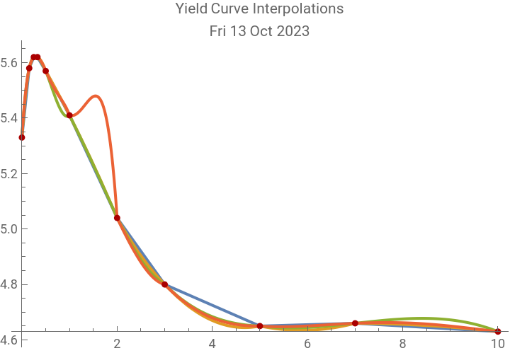


MonotonicInterpolation[], which has a continuous second derivative provides a less cyclic appearing interpolation than either the second or third order functions produced by Interpolation[]. Although the second derivative of the MonotonicInterpolation is continuous, it is not smooth. Adding a Chebyshev approximate polynomial gives a much smoother second derivative.
In[]:=
MonotonicInterpolation=ResourceFunction["MonotonicInterpolation"]
Out[]=
The following code creates monotonic interpolation, iFn, over seven weekly yield curves, looking at the first ten years of maturities. Functions are used from ChebyshevAlgorithms.m package which is included as an attachment. The coeffList will be used later in the notebook to analyze the curves. The Chebyshev approximation functions, yCurves, use ChebyshevT polynomial orders, {0, 10} .
In[]:=
?ChebyCoeff?ChebyFnD
Out[]=
Out[]=
In[]:=
iFn=MonotonicInterpolation[#]&/@crvs;coeffList=ChebyCoeff[#,{0,10},11]&/@iFn;yCurves=ChebyFnD[#,{0,10},11]&/@coeffList;
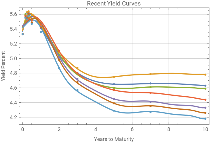
The plot below shows seven weekly Chebyshev polynomial approximate yield curves; the 13 Oct curve can be compared to the above plots to see that the MonotonicInterpolation[] input was smoother and less wavy, especially when there are long intervals between points. The data at one year and less do not fit well with the approximation, but years two through ten fit pretty smoothly, and these are the points which have been evolving. There is clearly a progressive change in the shapes of the curves, which will be looked at in more detail, using derivatives and lower orders of the Chebyshev polynomials.
In[]:=
ycp=PlotEvaluate[#[t]&/@yCurves],{t,0,10},;yclp=ListPlotEvaluate[crvs],;Show[ycp,yclp]
Out[]=


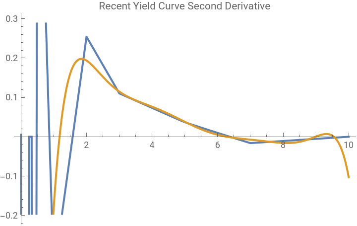
The Chebyshev polynomial approximation gives smooth derivatives, compared to the MonotonicInterpolation[], which although it can provide a continuous second derivative, that function is erratic and not smooth. The Chebyshev approximation removes the erratic behavior.
In[]:=
Plot{iFn[[1]]''[t],yCurves[[1]]''[t]},{t,0,10},
Out[]=
First derivative of the yield curve
First derivative of the yield curve
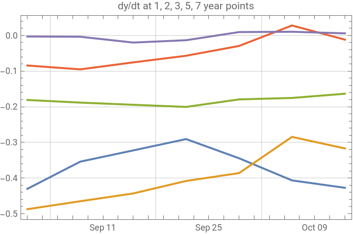
The current yield curve is inverted which means that for progressively increasing terms, the yields are declining. A normal yield curve should have rising rates for longer maturity terms to compensate for the increasing risk that rates may rise over time. The first derivative measures the slope of the curve. The following code looks at the first derivative at the {1, 2, 3, 5, 7} year nodes over the seven weeks of the data. The yield curve slopes will have to become positive for the shape of the curve to be normalizing; a normal yield curve should have all of the slopes positive. The graph shows that the longer term points are approaching the zero axis before the shorter maturity terms. The curve appears to be pulled up by the longer rates on the 6 Oct curve.
In[]:=
dydt1=#'[1]&/@yCurves;dydt2=#'[2]&/@yCurves;dydt3=#'[3]&/@yCurves;dydt5=#'[5]&/@yCurves;dydt7=#'[7]&/@yCurves;DateListPlot{Transpose[{recweek[[All,1]],dydt1}],Transpose[{recweek[[All,1]],dydt2}],Transpose[{recweek[[All,1]],dydt3}],Transpose[{recweek[[All,1]],dydt5}],Transpose[{recweek[[All,1]],dydt7}]},
Out[]=


Second derivative
Second derivative
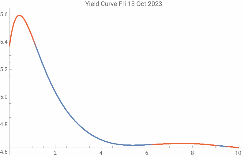
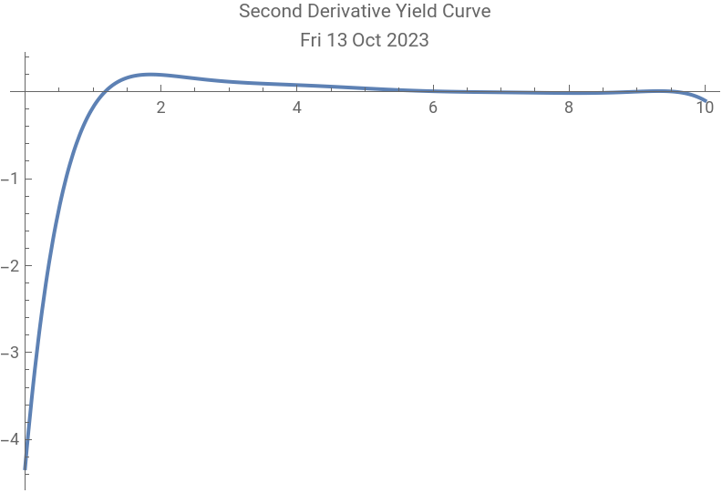
The concavity of the yield curve can be tracked by its second derive. A normal yield curve should be always concave downward. When the second derivative is negative the curve is concave downward. The red portions of the curve are concave downward by the second derivative.
In[]:=
Plot{yCurves[[1]][t]},{t,0,10},ColorFunctionFunction[{x,y},If[yCurves[[1]]''[x]<0,ColorData[97][4],ColorData[97][1]]],ColorFunctionScaling->False,Plot{yCurves[[1]]''[t]},{t,0,10},
Out[]=
Out[]=
For comparison a yield curve is constructed for data from 6 Jan 2022, which was about the time that equity markets peaked.
In[]:=
ycmp={0,0},,0.04`,,0.05`,,0.1`,,0.23`,{1,0.45`},{2,0.88`},{3,1.15`},{5,1.47`},{7,1.66`},{10,1.73`},{20,2.12`},{30,2.09`};ycmpCoeff=ChebyCoeff[MonotonicInterpolation[ycmp],{0,10},11];ycmpPoly=ChebyFn[ycmpCoeff,{0,10},11];
1
13
2
13
1
4
1
2
The red portion of curve is concave downward, which includes almost all of the first ten years.
Lower order Chebyshev polynomials
Lower order Chebyshev polynomials
After fitting to a higher order Chebyshev polynomial set, the coefficients of each ChebyshevT[n, x] order n can be looked at to give a general picture of some components of the shape. The 0th order coefficient gives a value in the mid range of the function. The sum of the the 0th and first order components gives the general trend of the curve. The sum of polynomial orders 0 through 2, determines the general convexity or concavity of the function. A normal yield curve should be concave downward.
This code shifts and scales the Chebyshev domain of [-1, 1] to the domain of the data, [0, 10]; a and b are the beginning and end points of the domain, the Chebyshev parameter in this example will be t.
The complete approximate function becomes the dot product of the shifted cPolys and the coefficients for the curves; it gives the same result within machine precision as the previously computed polynomial in yCurves.
This method can construct curves defined by accumulations of the lower orders. The first order shape comes from the sum of the 0th and 1st order cPolys, and gives the general trend of the curve. A normal yield curve should be always increasing, here the general trend of the first order approximation is downward. The plots do show the progression over time; the flattest slope was on 6 Oct and the next on 13 Oct. The earlier trends had steeper negative slopes.
The slopes can be numerically extracted and plotted; the trend was improving until the most recent week.
The second order polynomial shows the general convexity or concavity of the curve. The current curves are all convex downward; a normal shaped yield curve would be concave downward.
The third order polynomial begins to pick up other bends in the curve, but it is not clear that important characteristics in the shape of the curves are showing up at this level.
Local bends with maxima and minima show up where the points are further apart in time, and the locations of these can be found, but this is probably not very useful information.
Discussion
Discussion
I mentioned in the introduction that the parametric model in my previous post was producing unexpected results with the recent change in the yield curve. The curves from that model are shown below. The model shabe has a more idealistic appearance, but it cannot mathematically pick variation in the right tail of the curve, because it is based on a distribution function, the first derivative of which is always positive and greater in the middle of the curve than at the tails.
The recent daily c-parameters, which should be measuring the degree of inversion, are much higher and look like there was a shock to the market rather than the progressive change seen in the polynomial parameters.
It appears that the parametric model cannot provide useful information about the recent changes in the shape of the yield curve. Economists do not have a consistent model for inflation which can explain both the inflation of the 1970s and 1980s and the lack of inflation in the first two decades of the twenty-first century. The hope is that the yield curve will eventually normalize, but it is far from clear how that will evolve. Will inflation be halted and short term rates be pushed low while the longer term rates remain high? Will there be a recession that will force the Fed to reduce rates, and will it reduce them below the inflation rate? Is the economy growing fast enough that it can continue to grow with higher long term rates? Will geopolitical turmoil and wars cause prolonged stagflation? There are no good answers; it is not even clear whether the yield curve changes will be a leading or lagging macro-economic signal.
The Chebyshev polynomial approximation to a MonotonicInterpolation[] is completely data driven and can display changes in the general shape of the function. The strategy eliminates some of the current noise in the short term points. The polynomial approach yields smooth first and second derivatives which can be used to monitor how the shapes of the curves are evolving. Chebyshev polynomial approximations have the property that the coefficients of the higher order polynomials become progressively smaller very quickly, so that information about the general shape of the curve appears to be concentrated in the lower order polynomials. This approach can likely be applied to many other data problems. The included ChebyshevAlgorithms package has not been rigorously tested, so use it carefully and please let me know of any bugs.
The Chebyshev polynomial approximation to a MonotonicInterpolation[] is completely data driven and can display changes in the general shape of the function. The strategy eliminates some of the current noise in the short term points. The polynomial approach yields smooth first and second derivatives which can be used to monitor how the shapes of the curves are evolving. Chebyshev polynomial approximations have the property that the coefficients of the higher order polynomials become progressively smaller very quickly, so that information about the general shape of the curve appears to be concentrated in the lower order polynomials. This approach can likely be applied to many other data problems. The included ChebyshevAlgorithms package has not been rigorously tested, so use it carefully and please let me know of any bugs.
CITE THIS NOTEBOOK
CITE THIS NOTEBOOK
FOMC rates: Chebyshev polynomial approximation to yield curve
by Robert Rimmer
Wolfram Community, STAFF PICKS, October 15, 2023
https://community.wolfram.com/groups/-/m/t/3036618
by Robert Rimmer
Wolfram Community, STAFF PICKS, October 15, 2023
https://community.wolfram.com/groups/-/m/t/3036618