With[{data=NestList[EnergyExchangeAllNN[FixedEnergyExchange[True]],ConstantArray[1,1000],2000]},Histogram[Catenate[Take[data,-500]],Automatic,{"Log","Count"},ChartStyle$SecondLawColors["Blues",3],PlotRange->All,FrameTrue,AspectRatio1/3]]
Evolution
Evolution
In[]:=
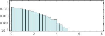
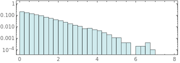
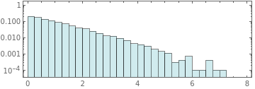
With[{data=NestList[EnergyExchangeAllNN[FixedEnergyExchange[True]],ConstantArray[1,10000],20]},Histogram[#,{.25},{"Log","Probability"},ChartStyle$SecondLawColors["Blues",3],PlotRange->{{0,8},{Automatic,1}},FrameTrue,AspectRatio1/3]&/@data]
Out[]=
,

,

,

,
,

,

,

,

,

,

,

,

,

,

,

,

,

,
,
,


In[]:=
GraphicsGrid[Partition[With[{data=NestList[EnergyExchangeAllNN[FixedEnergyExchange[True]],ConstantArray[1,10000],16]},Histogram[#,{.25},{"Log","Probability"},ChartStyle$SecondLawColors["Blues",3],PlotRange->{{0,8},{Automatic,1}},FrameTicks->None,FrameTrue,AspectRatio1/3]&/@data],4]]
Out[]=

In[]:=
8/30.
Out[]=
0.266667
In[]:=
GraphicsGrid[Partition[With[{data=NestList[EnergyExchangeAllNN[FixedEnergyExchange[True]],ConstantArray[1,10000],16]},Histogram[#,{.25},{"Log","Probability"},ChartStyle$SecondLawColors["Blues",3],PlotRange->{{0,8},{Automatic,1}},FrameTicks->None,FrameTrue,AspectRatio1/3]&/@data],4]]
Out[]=
In[]:=
GraphicsGrid[Partition[With[{data=NestList[EnergyExchangeAll[FixedEnergyExchange[True]],ConstantArray[1,10000],16]},Histogram[#,{.25},{"Log","Probability"},ChartStyle$SecondLawColors["Blues",3],PlotRange->{{0,8},{Automatic,1}},FrameTicks->None,FrameTrue,AspectRatio1/3]&/@data],4]]
Out[]=

In[]:=
GraphicsGrid[Partition[With[{data=NestList[EnergyExchangeAllNN[FixedEnergyExchange[True]],CenterArray[ConstantArray[100,100],10000],16]},Histogram[#,{.25},{"Log","Probability"},ChartStyle$SecondLawColors["Blues",3],PlotRange->{{0,8},{Automatic,1}},FrameTicks->None,FrameTrue,AspectRatio1/3]&/@data],4]]
Out[]=

In[]:=
GraphicsGrid[Partition[With[{data=Take[NestList[EnergyExchangeAllNN[FixedEnergyExchange[True]],CenterArray[ConstantArray[100,100],10000],1600],1;;-1;;100]},Histogram[#,{.25},{"Log","Probability"},ChartStyle$SecondLawColors["Blues",3],PlotRange->{{0,8},{Automatic,1}},FrameTicks->None,FrameTrue,AspectRatio1/3]&/@data],4]]

-308
10
-307
10
-308
10
Out[]=

Integer case
Integer case
Fixed energy distribution fractions
Fixed energy distribution fractions
One collision at a time...
[[[ Pure diffusion equation in energy space ]]]
Pure diffusion should approach uniform distribution.... [ others might be bimodal uniform ]
Weighted Pascal’s triangle.... [ but with wrapping ]
Initially uniform
Initially uniform
Random Connections
Random Connections
Actual hard spheres
Actual hard spheres