This notebook is part of the calculations that can be found in the book “Wave Optics in Infrared Spectroscopy - Theory, Simulation and Modelling”, to be published by Elsevier in autumn 2024. Here we calculate the reflectance of a dielectric material with arbitrary anisotropy following a scheme which is a mixture of the approaches provided by Berreman (D.W.Berreman,J.Opt.Soc.Am.62,502 (1972)) and Yeh (P.Yeh,J.Opt.Soc.Am.69,742 (1979)) as detailed in T. G. Mayerhöfer and J. Popp, Journal of Optics A: Pure and Applied Optics 8, 657 (2006). More details can be found in the book “Wave Optics in Infrared Spectroscopy - Theory, Simulation and Modelling”, to be published by Elsevier in autumn 2024.
Calculating a value of the dielectric tensor function at the wavenumber ν assuming a classical damped harmonic oscillator model (CDHO). The orientation of the transition moment of the oscillator is specified by spherical coordinates and the angles Phi and Theta. The CDHO model features three parameters, the oscillator strength , the damping constant and the wavenumber position . The tensor specifies a constant offset caused by oscillators with much higher oscillator position beyond a transparency region. It is the unity tensor if such oscillators and or transparency regions are not existing.
2
S
γ
νo
ϵ∞
Remove["Global`*"]ϵkk=Compile{{ν,_Real},{S,_Real,1},{γ,_Real,1},{νo,_Real,1},{ϵ∞,_Complex,2},{Phi,_Real,1},{Theta,_Real,1}},Module{Sm=S,γm=γ,νm=νo,ϵ∞m=ϵ∞},ϵ∞m+--Iγm[[i]]ν*
;
Length[Sm]
∑
i=1
2
Sm[[i]]
2
νm[[i]]
2
ν
2 (Sin[Theta[[i]]]*Cos[Phi[[i]]]) | (Sin[Theta[[i]]]*Cos[Phi[[i]]])(Sin[Theta[[i]]]*Sin[Phi[[i]]]) | (Sin[Theta[[i]]]*Cos[Phi[[i]]])*Cos[Theta[[i]]] |
(Sin[Theta[[i]]]*Cos[Phi[[i]]])(Sin[Theta[[i]]]*Sin[Phi[[i]]]) | 2 (Sin[Theta[[i]]]*Sin[Phi[[i]]]) | (Sin[Theta[[i]]]*Sin[Phi[[i]]])*Cos[Theta[[i]]] |
(Sin[Theta[[i]]]*Cos[Phi[[i]]])*Cos[Theta[[i]]] | (Sin[Theta[[i]]]*Sin[Phi[[i]]])*Cos[Theta[[i]]] | 2 Cos[Theta[[i]]] |
This uses one of the 24 different possibilities to specify the Euler angles according to T. G. Mayerhöfer, Spectrochim Acta A 61, 2611 (2005), to convert the dielectric tensor function from the internal coordinate system fixed inside the crystal to the laboratory coordinate system.
φ,θ,ψ
ϵ=Compile{{φ,_Real},{θ,_Real},{ψ,_Real},{ϵxx,_Complex},{ϵxy,_Complex},{ϵyy,_Complex},{ϵyz,_Complex},{ϵzz,_Complex},{ϵxz,_Complex}},Module{A},A=
;A.{{ϵxx,ϵxy,ϵxz},{ϵxy,ϵyy,ϵyz},{ϵxz,ϵyz,ϵzz}}.Inverse[A];
Cos[θ]Cos[φ]Cos[ψ]-Sin[φ]Sin[ψ] | Cos[θ]Cos[ψ]Sin[φ]+Cos[φ]Sin[ψ] | -Cos[ψ]Sin[θ] |
-Cos[ψ]Sin[φ]-Cos[θ]Cos[φ]Sin[ψ] | Cos[φ]Cos[ψ]-Cos[θ]Sin[φ]Sin[ψ] | Sin[θ]Sin[ψ] |
Cos[φ]Sin[θ] | Sin[θ]Sin[φ] | Cos[θ] |
This function calculates the so-called Δ-Matrix. Its input is the dielectric tensor function in laboratory coordinates ϵ and the wavevector k of the incidenct wave. In case of the latter it is assumed that the plane of incidence is the Y-Z-plane, so that only the Y component k[[2]] appears in the formula.
DD=Compile{{ϵ,_Complex,2},{k,_Complex,1}},
;
0 | 1 | 0 | 0 |
ϵ1,1- 2 k[[2]] ϵ1,3ϵ3,1 ϵ3,3 | 0 | ϵ1,2- ϵ1,3ϵ3,2 ϵ3,3 | -k[[2]] ϵ3,1 ϵ3,3 |
-k[[2]] ϵ3,1 ϵ3,3 | 0 | -k[[2]] ϵ3,2 ϵ3,3 | 1- 2 k[[2]] ϵ3,3 |
ϵ2,1- ϵ2,3ϵ3,1 ϵ3,3 | 0 | ϵ2,2- ϵ2,3ϵ3,2 ϵ3,3 | -k[[2]] ϵ2,3 ϵ3,3 |
Calculating the wavevector and the polarization of the two waves in the anisotropic medium.
EE[DD_]:=Eigensystem[DD];
Computing the so-called Dynamical Matrix of the anisotropic medium from the results of the eigensystem calculation.
GG[EE1_]:=Module{EEE=Table[{EE1[[1,i]],EE1[[2,i]]},{i,1,4}],FFF},FFF=DeleteCases[Table[If[Im[EEE[[i,1]]]≠0,If[Im[EEE[[i,1]]]>0,EEE[[i]],"a"],If[Re[EEE[[i,1]]]>0,EEE[[i]],"a"]],{i,1,4}],_String,2];
;
FFF[[1,2,1]] | 0 | FFF[[2,2,1]] | 0 |
FFF[[1,2,2]] | 0 | FFF[[2,2,2]] | 0 |
FFF[[1,2,3]] | 0 | FFF[[2,2,3]] | 0 |
FFF[[1,2,4]] | 0 | FFF[[2,2,4]] | 0 |
Calculating the Dynamical Matrix of the incidence medium and from the product of this matrix and the Dynamical Matrix of the anisotropic medium the M-Matrix that relates the amplitudes of the incident waves with those of the reflected and transmitted waves.
M2=Compile{{T,_Complex,2},{α,_Real},{n,_Complex}},ModuleLa=
,La.T;
1 2 | Sec[α] 2n | 0 | 0 |
1 2 | - Sec[α] 2n | 0 | 0 |
0 | 0 | Sec[α] 2 | 1 2n |
0 | 0 | - Sec[α] 2 | 1 2n |
Computing a common denominator needed for the calculation of the reflection and transmission coefficients.
Nenner=Compile[{{M,_Complex,2}},M[[1,1]]M[[3,3]]-M[[1,3]]M[[3,1]]];r=Compile{{M,_Complex,2},{NN,_Complex}},Module{r},{{M[[2,1]]M[[3,3]]-M[[2,3]]M[[3,1]],M[[4,1]]M[[3,3]]-M[[4,3]]M[[3,1]]},{M[[1,1]]M[[2,3]]-M[[2,1]]M[[1,3]],M[[1,1]]M[[4,3]]-M[[4,1]]M[[1,3]]}};
1
NN
Calculation of the reflectance based on the reflection coefficients.
R[r_]:=Chop[r*Conjugate[r]];
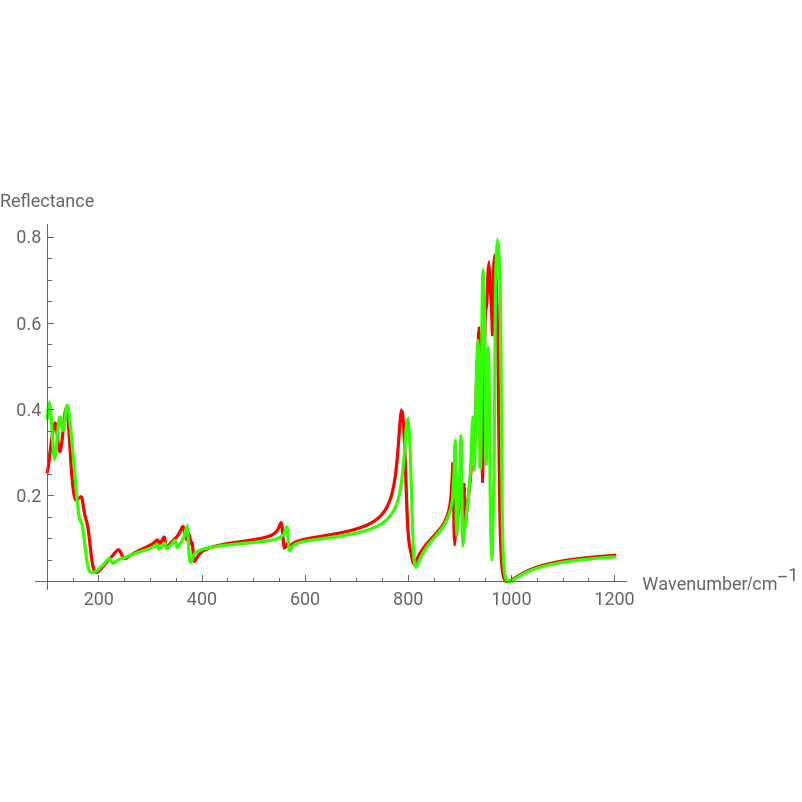
This function puts everything together and displays the reflectance spectra with s- and p-polarized incidenct light, as well as the ss- and pp-spectra and the cross-polarization terms sp and ps (spectra with polarized incident light and an analysator). If the variable Speichern equals the string “Ok”, it also saves these spectra. The parameter needed for the calculation are the angle of incidence , a list which specifies the wavenumbers at which the calculation is performed, the three Euler angles , the dielectric tensor function of the material specified in a coordinate system fixed inside the crystal and the refractive index of the isotropic and non-absorbing incidence medium.
α
φ,θ,ψ
ϵϵϵϵ
Berreman[α_,ν_,φ_,θ_,ψ_,ϵϵϵϵ_,n_,Speichern_]:=Module{pfff,kkin,ϵϵϵ,Rav,Rbv,zzz,äS,stream,methode},kkin=n{0,Sin[α],Cos[α]};pfff=Table[ϵϵϵ=ϵϵϵϵ〚ö〛;Rv=Module[{ϵϵ,EEE,GGG,Ma,NN,ra},ϵϵ=ϵ[φ°,θ°,ψ°,ϵϵϵ〚1,1〛,ϵϵϵ〚1,2〛,ϵϵϵ〚2,2〛,ϵϵϵ〚2,3〛,ϵϵϵ〚3,3〛,ϵϵϵ〚1,3〛];EEE=EE[DD[ϵϵ,kkin]];GGG=GG[EEE];Ma=M2[GGG,α,n];NN=Nenner[Ma];ra=r[Ma,NN];R[ra]];Rav=Rv〚1,1〛+Rv〚1,2〛;Rbv=Rv〚2,1〛+Rv〚2,2〛;{ν〚ö〛,Rav,Rbv,Rv〚1,1〛,Rv〚2,2〛,Rv〚2,1〛,Rv〚1,2〛},{ö,1,Length[ν]}];äS={"Rs","Rp","Rss","Rpp","Rps","Rsp"};zzz=Table[ListPlot[Table[{pfff〚i,1〛,pfff〚i,ü〛},{i,1,Length[pfff]}],PlotRangeAll,JoinedTrue,DisplayFunctionIdentity,PlotLegends{äS[[ü-1]]},AxesOrigin{ν〚1〛,0},PlotStyle{Hue[0.3`(ü-2)]}],{ü,2,7}];Table[Print[Show[zzz〚i〛,zzz〚i+1〛,DisplayFunction$DisplayFunction,PlotRangeAll,AxesLabel{"Wavenumber/","Reflectance"},ImageSize{1000,1000}]],{i,1,5,2}];IfSpeichernok,methode="Berreman.triklin.gold";SetDirectory["c:/Temp"];Forü=0,ü<Length[äS],stream=OpenWriteStringInsertäSü,StringInsertToStringmethode,N,3,N[φ,3],N[θ,3],N[ψ,3],".prn",-1,-1;For[i=0,i<Length[pfff],WriteString[stream,pfff〚i,1〛," \t ",pfff〚i,ü+"1"〛,"\n"],i++];Close[stream];,ü++;;
-1
cm
α
°
Oscillatorparameter of triclinic as obtained by dispersion analysis, S. Höfer, J. Popp, and T. G. Mayerhöfer, Vib. Spectrosc 72, 111 (2014).
K
2
Cr
2
O
7
Sx={74.5,78,111.5,80.2,106.6,130.4,85.3,112.1,93.3,87.7,97.5,107.2,53.3,32.8,50.9,23,23.3,33.5,27.6,31.9,63.3,79.9,86.1,105.4,39.7,32.5,41.4,75,72,513.7,300.3,147.6,146.7,153.2,89.7,223.9,119.2,368.8,280.3,157.4,196.4,256.7,133.9,134.7};γx={11.2,7.8,9.7,10.2,14.6,12.7,11.7,14.6,13.3,48.8,17.8,20.4,10.2,10.1,16.1,4.7,6.2,5.6,4.6,5.2,6.3,11,5.9,9.4,5.4,2.4,5.3,7.1,5.1,11.3,8.4,3,2.4,2.8,2.9,2.8,3.6,3.3,4,2,3.8,1.2,4.2,1.2};νx={88.9,89,103.8,105.7,114.8,121.6,129.5,132.3,135,155.8,157.3,162.4,165.8,222.6,241.9,314.2,315.4,328.2,329.6,349.3,363.7,366,371.6,375,375.8,377.4,381.5,555.5,566,742.4,792.7,883.2,889.7,901.4,908.3,921.6,926,928.6,936.7,942.1,947.3,947.6,955,965.5};phi={8.1,174.2,83.1,42.8,7,107.6,4.2,24,82.3,98.3,0.6,167.1,133.9,79.7,161.9,86.2,177.7,170.6,72.1,81,15,158.7,73.9,156.2,164.1,179.7,15.3,179.6,112.6,48.1,133.4,12.1,122,123.5,21,1.1,115.1,54.4,137,73.8,178.7,85.1,16.7,109.8}°;theta={92.1,23.8,92.1,52.4,98.5,106.9,25.3,91,86.1,90.6,176.5,56.3,95.8,79.6,92.1,94.6,89.3,78.5,72,102,26.6,48.3,56.6,155.3,98.1,5.5,95.3,93.3,92.7,31.3,80.5,22.7,68,77.1,82.1,130.7,100.7,105.6,82.1,70.9,95,133.8,51.4,100.8}°;ϵ∞xx=3.02;ϵ∞yy=3.41;ϵ∞zz=2.54;ϵ∞xy=0.01;ϵ∞xz=0.09;ϵ∞yz=0.01;ϵ∞={{ϵ∞xx,ϵ∞xy,ϵ∞xz},{ϵ∞xy,ϵ∞yy,ϵ∞yz},{ϵ∞xz,ϵ∞yz,ϵ∞zz}};ϵ∞={{ϵ∞xx,ϵ∞xy,ϵ∞xz},{ϵ∞xy,ϵ∞yy,ϵ∞yz},{ϵ∞xz,ϵ∞yz,ϵ∞zz}};
List with wavenumber points.
ν1=Range[100,1200,1];
Generating the dielectric tensor function.
ϵϵϵϵϵ=Table[Chop[ϵkk[ν1[[ö]],Sx,γx,νx,ϵ∞,phi,theta]],{ö,1,Length[ν1]}];
Program execution.
Berreman[20°,ν1,0,0,0,ϵϵϵϵϵ,1,o]


CITE THIS NOTEBOOK
CITE THIS NOTEBOOK
Calculating reflectance of anisotropic crystals with a 4x4 matrix formalism
by Thomas Mayerhöfer
Wolfram Community, STAFF PICKS, May 16 2023.
https://community.wolfram.com/groups/-/m/t/2920841
by Thomas Mayerhöfer
Wolfram Community, STAFF PICKS, May 16 2023.
https://community.wolfram.com/groups/-/m/t/2920841