This computational essay investigates one-dimensional super-oscillations, demonstrating how band-limited functions can locally exceed their highest constituent frequencies. We trace this phenomenon from M. V. Berry’s famous example of a super-oscillatory function, then analyze super-oscillatory behavior in one-dimensional quantum wavefunctions (the particle in a box and the harmonic oscillator). Furthermore, we address the physical reality of leaky functions: because real-world spectra are almost always leaky, strict mathematical super-oscillations often do not exist, yet we demonstrate how one can still meaningfully analyze fast oscillations within localized zones. Finally, we include band-limited Slepian functions as an additional example.
Introduction
Introduction
Super-oscillations are a mathematical phenomenon where a band-limited function oscillates faster than its highest constituent frequency component within a specific local interval. In simpler terms, if you have a signal made only of low-frequency waves, a super-oscillatory segment of that signal can appear to be a high-frequency wave. This seems to defy the intuitive understanding of the Fourier band-limit, which suggests that a function cannot wiggle faster than its fastest component.
For a function, which is typically complex-valued in these contexts, the local wave-vector (x) represents the spatial rate of change of the function’s phase. It is defined for a 1D function as:
For a function
f
k
local
k
local
x
x
f
Or if we express the function as then we see (x)= is the gradient of the phase. If the function is band-limited by a in its Fourier transform, a region of super-oscillation is denoted for points where |(x)|
f(x)=A(x)
ϕ(x)
k
local
ϕ(x)
x
k
max
x
k
local
>
k
max
Show that the definition of is the gradient of the phase:
k
local
In[]:=
Im//ComplexExpand//FullSimplify
DA[x],x
ϕ[x]
A[x]
ϕ[x]
Out[]=
′
ϕ
And the real part of the logarithmic derivative is related to amplitude change:
In[]:=
Re//ComplexExpand//FullSimplify
DA[x],x
ϕ[x]
A[x]
ϕ[x]
Out[]=
′
A
A[x]
Berry’s function
Berry’s function
A key example of super-oscillations studied by Michael Berry and based on work with Yakir Aharonov is the function
f(x)=(Cos(x/N)+a
N
Sin(x/N))
It is stated that the function presents super-oscillations for and . This prototype function is periodic
f
a>1
N>>1
Nπ
Define the Berry super-oscillatory function:
In[]:=
f[x_,a_,N_]:=
N
(Cos[x/N]+aSin[x/N])
Calculate the symbolic local wave-vector:
In[]:=
kLocal=Im//ComplexExpand//FullSimplify
D[f[x,a,n],x]
f[x,a,n]
Out[]=
a
2
a
2
sin
x
n
2
cos
x
n
Symbolic local growth rate, or in other words is the local rate of amplitude change:
In[]:=
κ=Re//ComplexExpand//FullSimplify
D[f[x,a,n],x]
f[x,a,n]
Out[]=
-
(-1)sin
2
a
2x
n
(-1)cos--1
2
a
2x
n
2
a
The Berry’s function is band-limited, the magnitude of their wave-vector components are all less than 1
Sample an integer for the value of :
N
In[]:=
Nsample=RandomInteger[{1,50}];
Calculate the values present in the function:
k
n
In[]:=
Union@@Cases[FourierTransform[f[x,a,Nsample],x,k],DiracDelta[a_]:>SolveValues[a==0,k],∞]
Out[]=
-1,-,-,-,-,-,-,-,-,-,-,-,-,-,,,,,,,,,,,,,,1
25
27
23
27
7
9
19
27
17
27
5
9
13
27
11
27
1
3
7
27
5
27
1
9
1
27
1
27
1
9
5
27
7
27
1
3
11
27
13
27
5
9
17
27
19
27
7
9
23
27
25
27
The general result is =-1+2n/N, so || :
k
n
k
max
=1
In[]:=
Array[-1+2#/Nsample&,Nsample+1,0]
Out[]=
-1,-,-,-,-,-,-,-,-,-,-,-,-,-,,,,,,,,,,,,,,1
25
27
23
27
7
9
19
27
17
27
5
9
13
27
11
27
1
3
7
27
5
27
1
9
1
27
1
27
1
9
5
27
7
27
1
3
11
27
13
27
5
9
17
27
19
27
7
9
23
27
25
27
Test the equality, we see indeed is band-limited:
In[]:=
(%==%%)
Out[]=
True
N=20,a=6
N=20,a=6
There is a super-oscillation zone centered at , the local wave-vector exceeds the maximum wave-vector and the growth rate tends to 0 when :
x=0
x->0
In[]:=
PlotEvaluate[{kLocal,κ,1,-1}/.{a->6,n->20}],{x,-40,40},
Out[]=
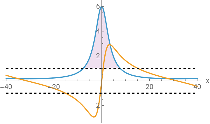


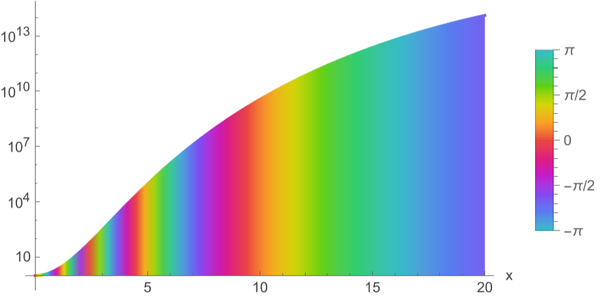
Super-oscillations are notorious when approaching , but nothing is free to get those high-frequency oscillations in the “zone,” the price to pay is to get the magnitude of the function gets exponentially smaller
x=0
Magnitude and phase plot:
AbsArgPlotf[x,6,20],{x,0,20},
Out[]=
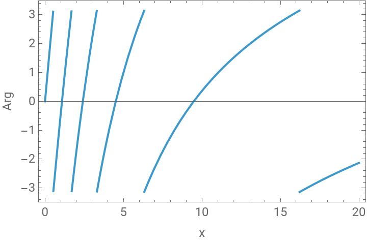
More pronounced Arg slopes:
In[]:=
PlotArg[f[x,6,20]],{x,0,20},
Out[]=
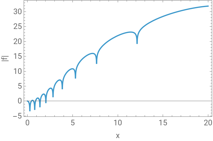
Increased frequency in the magnitude oscillations:
In[]:=
PlotLog@Abs@Re[f[x,6,20]],{x,0,20},
Out[]=
N=10,a=0.999
N=10,a=0.999
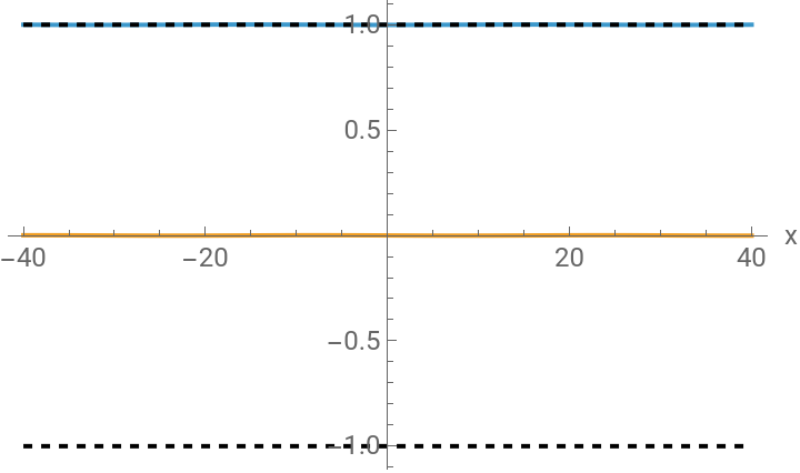
For this value of , we are not supposed to get super-oscillations:
a
In[]:=
PlotEvaluate[{kLocal,κ,1,-1}/.{a->0.999,n->10}],{x,-40,40},
Out[]=
Visualize the amplitude and phase:
In[]:=
Plot[Log@Abs@Re[f[x,0.999,10]],{x,-10,10},PlotRange->All]
The chosen values generate an extension of the super-oscillation zone:
And it is interesting to observe the super-oscillations do not occur in the interval where the wave-function varies more:
Particle in a box wave-functions
Particle in a box wave-functions
While pure super-oscillations are, by definition, produced by band-limited functions (like sums of sines), they can be extended to “leaky” functions that have infinite bandwidth. A function is considered to have super-oscillations if it has a mostly low-frequency spectrum, with an extremely faint “tail” of high-frequency components that do not contribute to the overall amplitude but are responsible for rapid local variations. These can be called “quasi-super-oscillations.” , they are indistinguishable locally from true super-oscillations but lack the strict band-limited guarantee.
Two state superposition
Two state superposition
No relative phase
No relative phase
Define a two state superposition:
But it is highly concentrated in the values close to 5π and 6 π :
With relative phase
With relative phase
Two state superposition using a relative phase:
And those zones are related to an increased phase gradient:
But it is interesting to note this is not reflected in the real and imaginary parts of the wave-function, that oscillate with the given frequencies of the sine wave-functions:
More superpositions
More superpositions
Balanced superposition
Balanced superposition
Define a uniform superposition:
Calculate the Fourier transform:
Also as expected for this case there are also no super-oscillations:
Binomial coefficient superposition
Binomial coefficient superposition
Consider a more complicated superposition with complex coefficients:
Build ψ(x):
Fourier transform:
Local wave-vector
Observing the phase tells us there is a change of behavior in the local wave-vector peaks, but they are not notorious enough:
Engineering super-oscillations
Engineering super-oscillations
Sampling around the target zone:
Get the function evaluations:
Solve for the coefficients:
Engineered wavefunction:
Calculate its Fourier transform:
The local wave-vector gives us no useful information since the wave-function are real and the coefficients are also real:
But we can calculate the real part of the logarithmic derivative to get information in the change of amplitude:
This quantity has oscillations with high amplitude in the target zone:
Visualize the oscillations in the amplitude of the wave-function in the restricted zone:
Harmonic Oscillator
Harmonic Oscillator
Quantum harmonic oscillator wave functions:
Maximum k as energy content integral
Maximum k as energy content integral
Fraction of total integral for some finite symmetric region:
Method 2 (energy integral)
Method 2 (energy integral)
Vary the precision:
Method 3
Method 3
Use this estimation for the other methods:
Two state superposition
Two state superposition
If we consider a superposition with real coefficients the local momentum will be clearly 0, so we define a superposition with relative phase:
Local momentum:
Show super-oscillatory region, which are very localized peaks:
Many wave functions superposition
Many wave functions superposition
Build wavefunction:
Local wave-vector:
Show super-oscillations zone:
Plot real and imaginary part:
We also see in this case fast phase changes in zones where |ψ| goes to zero, that of course correspond to the potential super-oscillations peaks:
Target super-oscillations zone
Target super-oscillations zone
We can follow a similar approach when using the particles in a box wavefunction to try to design super-oscillations
Set up parameters:
Build the design matrix:
Obtain the coefficients using least squares and normalize them:
Construct the wavefunction:
Visualize the super-oscillation zone:
Zoom of the super-oscillation candidate zone:
Leaky Prototype function
Leaky Prototype function
Define the leaky function:
When β ≠0, the Fourier series terms can be increased as much as needed,showing is not band-limited:
Phase and magnitude plot:
Increased rate of change of the phase when approaching the super-oscillation zone:
Monochromatic waves
Monochromatic waves
In one dimension the elementary scalar wave is
Two wave model
Two wave model
Define a two wave model that depends on a parameter ε :
Local wave-vector:
However if we take a small value of ϵ that is not zero we can observe interesting behavior
High phase gradient in the peaks:
Magnitude and Arg zoom plot in one of the zones:
Many waves
Many waves
Definition for the sum of plane waves:
Plot the real part, imaginary part and the absolute value of the function:
Super-oscillations fraction or probability that an infinitesimal region has super-oscillations:
Find a super-oscillating peak:
Plot the phase close to the peak , we see there is a faster change in the phase:
Visualize more zones of fast phase change:
Prolate Spheroidal Functions
Prolate Spheroidal Functions
Plot the spheroidal function, we see the higher amplitude oscillations are concentrated in some zone:
Superposition
Superposition
Plot the local wave-vector:
We see the small zones of fast phase change that reflect the many super-oscillation peaks:
Conclusions
Conclusions
◼
Super-oscillations may manifest directly in the real or imaginary components(or the magnitude) , depending on the specific superposition or function family utilized. Alternatively, they can be identified as regions of high phase gradients, typically occurring where the magnitude approaches a local minimum or zero
◼
By applying these principles to fundamental quantum systems—such as the particle in a box and the harmonic oscillator—we demonstrated the ability to engineer super-oscillations in localized zones. Notably, these were designed to manifest as rapid amplitude fluctuations rather than a pronounced phase gradient
Utilities
Utilities
References
References
◼
Berry, M. V. (2013). Five momenta. European Journal of Physics, 34(6), 1337-1348.
◼
Berry, M. V. (2019). Super-oscillations and leaky spectra. Journal of Physics A: Mathematical and Theoretical, 52(1), 015202.
◼
Berry, M. V., & Dennis, M. R. (2009). Natural super-oscillations in monochromatic waves in D dimensions. Journal of Physics A: Mathematical and Theoretical, 42(2), 022003.
CITE THIS NOTEBOOK
CITE THIS NOTEBOOK
Superoscillations Part I: 1D foundations, leaky functions and quantum wavefunctions
by Bruno Tenorio
Wolfram Community, STAFF PICKS, May 9, 2026
https://community.wolfram.com/groups/-/m/t/3713462
by Bruno Tenorio
Wolfram Community, STAFF PICKS, May 9, 2026
https://community.wolfram.com/groups/-/m/t/3713462