The second fundamental theorem of Calculus.Larson Hostetler Edwards Calculus sixth ed pg. 280
b
∫
a
x
∫
a
“To avoid the confusion of using x in two different ways we temporarily switch to t”
There is a circle of understanding in the above of two equations. They are text and not active code. Before computers the same struggle to choose the letters and symbolism were also an issue! Written on paper with feathers and ink, sent by horseback and sail ship to mathematicians around the world, the problem was how to write the formulas in a conventional way that also kept the rigorous logic and computations intact. Consider the capitalization (upper case) of the F . Like a proper noun, capitol (upper case) F was understood as function like f ( lower)but also a name, or more strictly a title in an hierarchy of sentence structure. After exploring page 280, I purposed myself then to construct one simple elegant line of code that will capture the story being told, and perhaps one more for the picture. In this case the authors (textbook giants) ask for a plot to be made on CAS software of “for” (exact words) 0 ≤ x ≤ π Evaluated at 0, π/6, π/4, π/3, π/2. Then, an explanation of any expectations or whether or not it would look familiar. I think they, Hostedler Edwards and Larson, were assuming a math student might be surprised to see trapezoids and not a smooth sine curve . If all they want is an answer . . .
F(x)=cos(t)t
x
∫
a
f[x_]:=Cos[t]t[{0,π/6,π/4,π/3,π/2}]
x
∫
0
The list {0,π/6,π/4,π/3,π/2} is also enclosed in brackets and there is no comma after the differential operator t. That was a welcome surprise. Generally these code lines are very critical on any CAS and very sensitive to commas brackets and braces and the placement or order of elements inside of lists! f[x], {x,0,pi} “the function of x as x goes to pi” or this . . . f[x], {x , 0, 5, .2 } “f of x goes 0 to 5 in steps of 2 tenths”. Observe removing the list and brackets leaves . The original graph asked for.
f[x_]:=Cos[t]t
x
∫
0
Functionx,Cos[t]t[{0,π/6,π/4,π/3,π/2}]
x
∫
0
0,,,,1
1
2
1
2
3
2
ShowListLinePlot0,,,,1,PlotStyleRGBColor[0.96,1.,0.89],PlotTheme"Detailed",MeshAll,BackgroundBlack
1
2
1
2
3
2
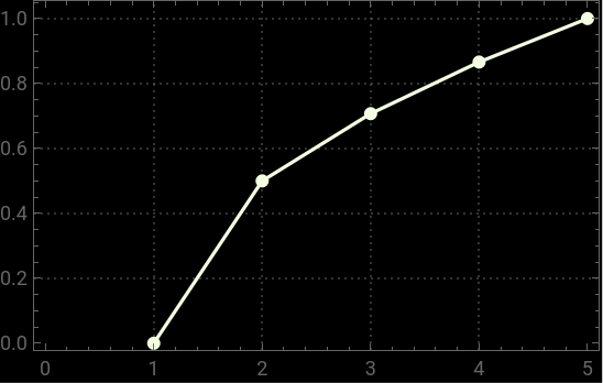
A bit strange the RGBColors. I seriously doubt anyone types these things in as opacity and hundredths of different shades of blue green and red. This is just point and click options. A black background and white line plot (including the points) produced [0.96,1.,0.89] which to me does not describe white. Not that I care since I am technically colorblind, but after reading the wolfram documentation, and also being a chemist, it just looks like all colors are at pretty much full power (especially the green coming in at full 1 (which I thought meant it would be “clipped”) and how exactly does that equal white? I remain dumbfounded at Show. Without it the line would appear but the data points would not. Does not Mesh ⟶All do that? Then why do I need Show?