This notebook looks at volatility of SPY ETF over the most recent 15 years. See a simple intraday volatility measure. Equity market volatility is not a random process, periods of high and low volatility tend to cluster in runs. It turns out that long run lengths of above median volatility are historically rather frequent. When long high volatility runs occur, they are associated with periods of market decline, but the analysis below shows that when a long run of above median volatility breaks, it may signal improvement in market returns. In this analysis it only takes one point of below 15-year median market volatility to break a high volatility run.
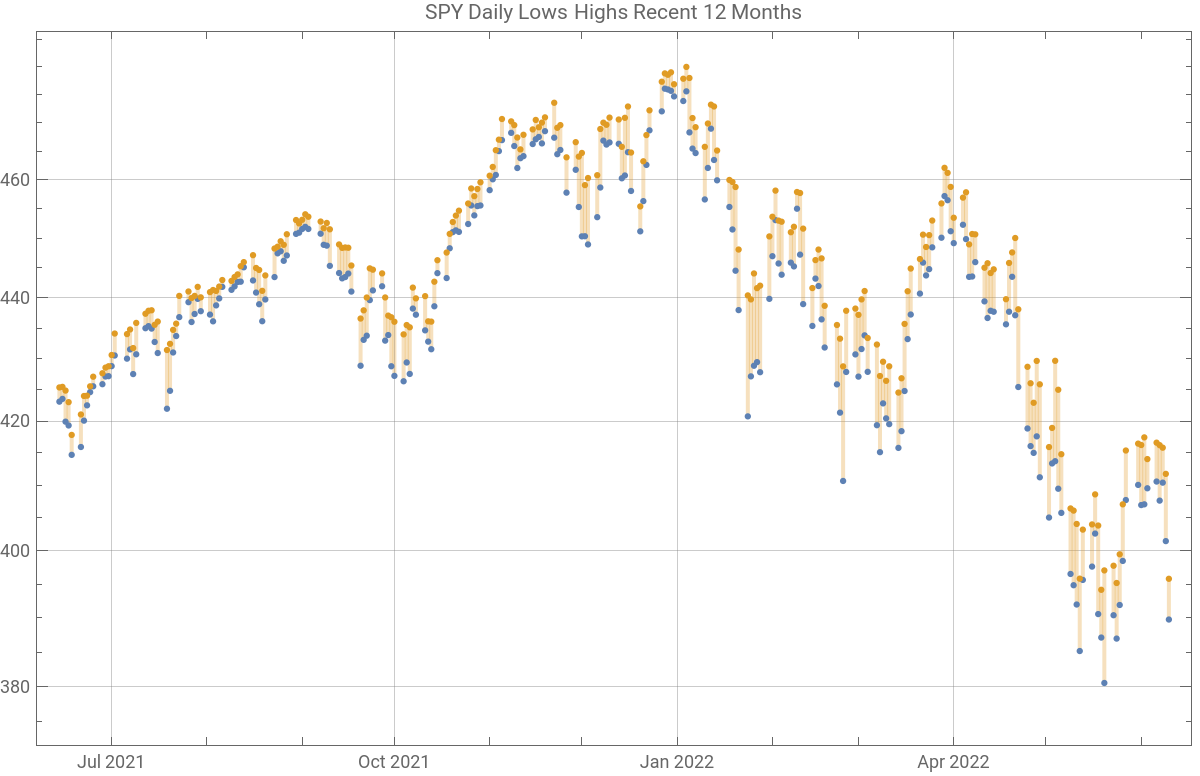
In the first graph below the blue and orange points are the daily low and high prices. The volatility graph is simply the log of the ratio of the high/low price each day. The current run of volatility above the median has only a very few breaks of volatility less than the median.
Initialization code
In[]:=
startDate=DatePlus[DateList[][[;;3]],{-15,"Year"}]{2007,6,12}data0=FinancialData["SPY","OHLCV",startDate];data={#1,QuantityMagnitude/@#2}&@@@Normal[data0];data[[-1]]
Out[]=
{2007,6,12}
Out[]=
{2007,6,12}
Out[]=
,{394.88,395.778,389.75,389.8,132893864}
In[]:=
loghilo={#1,Log[#2[[2]]/#2[[3]]]}&@@@data;edf=EmpiricalDistribution[loghilo[[All,2]]];Last[loghilo][[2]]CDF[edf,%]
Out[]=
0.015348
Out[]=
0.73882
In[]:=
q1=Quantile[edf,0.1]q5=Quantile[edf,0.5]q9=Quantile[edf,0.9]
Out[]=
0.00449442
Out[]=
0.00989824
Out[]=
0.024708
In[]:=
ygrid=Table[i,{i,0.01,Max[Take[loghilo[[All,2]],-252]]+0.01,0.01}]
Out[]=
{0.01,0.02,0.03,0.04,0.05}
In[]:=
DateListLogPlot{Tooltip[#,#]&/@({#1,#2[[3]]}&@@@Take[data,-252]),Tooltip[#,#]&/@({#1,#2[[2]]}&@@@Take[data,-252])},DateListPlot{Tooltip[#,#]&/@Select[Take[loghilo,-252],#[[2]]>q5&],Tooltip[#,#]&/@Select[Take[loghilo,-252],#[[2]]<q5&]},
Out[]=


Out[]=
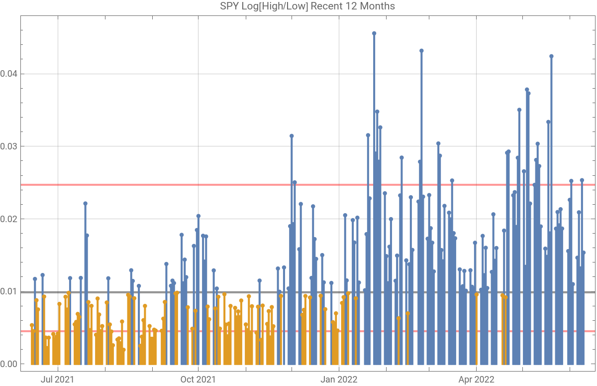
The 15 year median is the black line in the volatility chart. The red lines are the 0.1 and 0.9 quantiles. The peak price point of the SPY ETF occurred on 4 Jan 2022, a volatility spike occurred on 5 Jan 2022; since then U.S. equity markets have been in decline. Volatility has been above median for all but a few days since the volatility spike on 5 Jan. The rest of this notebook looks at the volatility signal in terms of run lengths above and below the median to see if the data contains any potentially useful information to predict the continuation or end of a run. The data set contains two previous market crashes; the current data could be the beginning of a third crash. The current economic factors are totally different from previous crash events, but financial markets have limited response patterns to information, i.e. prices can go up or down in varying magnitudes. Even though the economic parameters may be very different, price patterns will likely repeat.
Run lengths
Run lengths
The total number of days in the 15 year series.
In[]:=
Length[loghilo]
Out[]=
3779
Here a run consists of sequential volatility points either above or below the 15-year median.
In[]:=
runs=Split[loghilo,(#1[[2]]>=q5&[[2]]>=q5)||(#1[[2]]<q5&[[2]]<q5)&];
Probabiity of latest run length of volatility greater than median, if volatility were an independent random process.
In[]:=
runLengths=Length/@runs;%[[-1]]2^-%
Out[]=
36
Out[]=
1
68719476736
Long run lengths occur frequently.
In[]:=
Tally[runLengths]//Sort
Out[]=
{{1,446},{2,178},{3,74},{4,53},{5,49},{6,23},{7,21},{8,18},{9,12},{10,9},{11,8},{12,7},{13,7},{14,2},{15,8},{16,5},{17,5},{18,2},{19,2},{20,1},{21,1},{22,2},{23,1},{25,1},{27,1},{28,1},{29,1},{30,2},{31,1},{34,1},{35,1},{36,1},{37,1},{43,1},{52,1},{55,1},{61,1},{64,1},{66,1},{91,1},{139,1}}
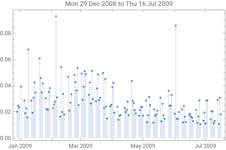
The longest run in the timeseries marked the end of the 2008 crash and beginning of the recovery. Notably after it ended equity markets rose for more than three years. Prior to this run breaking, volatility seemed to be generally declining.
In[]:=
longestRun=Select[runs,Length[#]==139&][[1]];DateListPlotlongestRun,
Out[]=
A listing of longer runs of volatility higher than median, including current run.
In[]:=
DateString[#[[1]][[1]],"DateShort"]<>" to "<>DateString[#[[-1]][[1]],"DateShort"]<>" Length "<>ToString[Length[#]]&/@Select[runs,Length[#]>=36&&#[[1]][[2]]>q5&]//TableForm
Out[]//TableForm=
Fri 4 Jan 2008 to Mon 7 Apr 2008 Length 64 |
Tue 24 Jun 2008 to Thu 14 Aug 2008 Length 37 |
Mon 18 Aug 2008 to Wed 24 Dec 2008 Length 91 |
Mon 29 Dec 2008 to Thu 16 Jul 2009 Length 139 |
Wed 27 Jul 2011 to Thu 27 Oct 2011 Length 66 |
Mon 24 Feb 2020 to Wed 6 May 2020 Length 52 |
Thu 21 Apr 2022 to Fri 10 Jun 2022 Length 36 |
Long runs of bellow median volatility are shorter.
In[]:=
DateString[#[[1]][[1]],"DateShort"]<>" to "<>DateString[#[[-1]][[1]],"DateShort"]<>" Length "<>ToString[Length[#]]&/@Select[runs,Length[#]>20&&#[[-1]][[2]]<=q5&]//TableForm
Out[]//TableForm=
Wed 2 Jan 2013 to Fri 1 Feb 2013 Length 22 |
Fri 31 Oct 2014 to Fri 5 Dec 2014 Length 25 |
Thu 29 Dec 2016 to Mon 20 Mar 2017 Length 55 |
Fri 30 Jun 2017 to Wed 9 Aug 2017 Length 28 |
Wed 6 Sep 2017 to Thu 30 Nov 2017 Length 61 |
Tue 5 Dec 2017 to Fri 12 Jan 2018 Length 27 |
Fri 3 Aug 2018 to Wed 3 Oct 2018 Length 43 |
Thu 28 Mar 2019 to Tue 30 Apr 2019 Length 23 |
Fri 11 Oct 2019 to Fri 29 Nov 2019 Length 35 |
This is the longest run of volatility below median in the series.
Long run lengths cluster.
Occurrence of run lengths greater than 25.
About 23% volatility points are in clusters of longer runs than 25 trading days.
In graph above the third and the current cluster contain short breaks in the cluster. Thus not every break in a long run signals the end of a period of high volatility, but a single point below median volatility marked the end of the other long runs of high and low volatility in the chart above.
Here is a look at the volatility through the COVID crash and recovery.
Conditional probability of run continuing
Conditional probability of run continuing
The sequence of volatility events has strong autocorrelation.
This is an attempt to calculate the conditional probability of a run continuing once it has started from the volatility data using the formula:
The algorithm below takes as input a list of ones and zeros as binary input. The algorithm specifically then looks at runs of ones in the list by sequentially partitioning the list. If the partition length is equal to the total of the partition, then the partition must contain all ones. The algorithm resamples the data many times so any errors in the probability estimate will propagate, but it performs reasonably well when given a pseudorandom sample putting out the expected result. The calculated sequential probabilities for the volatility series are of the order of magnitude needed to produce long runs.
Convert the volatility list to a sequence of 1s and 0s, where 1 is volatility ≥ median.
The graph shows the estimate of conditional probability that the run will continue at each current run length.
Calculate sequential probabilities that runs below median will continue.
Test the algorithm on pseudorandom data . This may be run repeatedly, it generally gives results close to the expected 0.5 for more than the first half of the run lengths in the sample.
Conclusions
Conclusions
This notebook has looked at run lengths above and below a median volatility measure to see if anything can be learned about the dependent structure of volatility. If run lengths above and below median were independent then the probability of a run length would be the same as the run lengths of heads or tails in a fair coin toss, 2^-n, where n would be the run length. And at each new data point, the probability of the run breaking would be 1/2.
The conditional probability calculations suggest the probability of the current run continuing should be more than 97% on the next trading day.
The conditional probability calculations suggest the probability of the current run continuing should be more than 97% on the next trading day.
The data set has 9 run lengths longer than the current, and the data set contains only two crashes, so there is not a lot of historical information for calculations. So probability estimates are not likely to be highly accurate.
But when high volatility runs break, a market recovery appears to be underway, for the two crashes in the data. With the SPY data a long run will frequently break and not restart. Thus lower than median volatility may have predictive value. It only takes changing a couple of lines of code in this notebook to run it with the VIX index downloaded from Yahoo; I will include this as an attachment. The VIX index is serially smoother, has fewer break points, and much longer runs, as well as about twice the autocorrelation, so it initially appears to be less useful to look for change points. Its distributional shape is not nearly so clean as the SPY volatility.