This notebook series is designed to introduce selected dynamic economic models to both advanced undergraduate and graduate students. Economists have relied on a series of economic models to better understand the otherwise highly complex causal relationship among many economic variables. Dynamic economic models set up by systems of either difference or differential equations are particularly useful in tracing the change in the quantity of unknown economic variables (e.g., the capital stock, demand for labor, aggregate output, etc.) and their interactions over time.
This notebook series aims to help students better understand the depth, usefulness, and limitations of major existing micro and macroeconomic models by demonstrating how we can use Wolfram Mathematica to replicate and reconstruct the core ideas and find dynamic solution of the model.
The model introduced in this notebook series include, among others, (1) the cobweb model of the quantity and price adjustment, (2) Keynes’s aggregate demand model, (3) Hicks’s ISLM model, (4) Samuelson’s investment accelerator model, (5) Kalecki’s investment delay model, (6) the predator-prey interaction model, (7) the epidemic model, (8) Ricardo’s three dimensional business cycle model, (9) Marx-Goodwin business cycle and growth model, (10) Smith’s and Ricardo’s growth model, (11) the Harrod-Domar growth model, (12) the Solow growth model, (13) the RBC model, (14) Romer’s new growth model, and (15) the circuit of capital model.
Introduction
Introduction
We have learned so far how we can use Wolfram Mathematica to build and replicate major macroeconomic and business cycle models in a dynamic setting. We have also learned how we can find and visualize the solution to a system of difference and differential equations used in economic analysis.
Both difference and differential equation allow us to trace changing value of a solution function defined by the model. The change in the productive capital stock and the change in the economy’s aggregate productive capacity measured by aggregate output-income are the prime examples in this part of analysis.
From now on, we will turn our focus onto the analysis of long-run economic growth and growth models. The economic growth models we will examine include (1) the Harrod-Domar growth model, (2) the Solow growth model, (3) the real business cycle (RBC) model, (4) the Romer endogenous growth model, and (5) the circuit of capital model.
As a starter, this note provides an overview of various growth processes. There are at least three interesting growth patterns that are relevant to our discussion. These are (1) the exponential growth pattern, (2) the exponential growth with an upper limit, and (3) the logistic growth pattern. After briefly presenting these three growth patterns, we also reconstruct both Adam Smith and David Ricardo’s respective ideas about the economic growth process. The analysis in this part will provide a useful reference point for various economic growth models that come later.
Three growth patterns
Three growth patterns
The exponential growth
The exponential growth
Most economic models involves the rate of change or growth rate of a certain quantity such as the aggregate output-income measured by GDP or the growth of a fixed capital stock. Unless specified otherwise, these changes are typically represented by the exponential growth model.
As an example, let X(t) denote an economic variable such as the GDP of a country or a unit of productive capital stock. The ratio (t)/X(t) is the rate of change in this quantity. Several economic models postulate that the growth rate of a certain quantity is approximately a constant, r. Thus, we can say that the change in the quantity of this variable is stated by a differential equation, (t) = r X(t) for all t.
X
X
If r = 1, this equation becomes (t) = X(t), and its general solution is X(t) = A where A is an arbitrary constant. If r ≠ 1, then we get x(t) = A as a solution for (t) = r X(t). If the value of X(t) at t, X(0) is given by X0, then X0 = A = A. Therefore, we can conclude that the solution to the differential equation (t) = r X(t) with its initial value X(0) = X0 is x(t) = X0. If the initial value of the stock is given, the problem of finding the solution to this equation becomes an initial value problem.
X
t
rt
X
0
X
rt
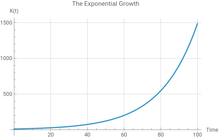
Let us use this idea to solve the following questions: Let K(t) denote a fixed capital stock of a business enterprise at time t. Ignoring depreciation of this capital stock, net investment will increase the volume of this capital stock over time at a constant proportional rate, a (a > 0), implying that (t) = aK(t) or (t) /K(t) = a.
K
K
Let us (1) find an expression for K(t) when the capital stock at time 0 is K0. And (2) solve the equation K0 = K0 for t. That is the time when the capital stock doubles the amount of its initial value.
at
2
(1) The solution to the first question is K(t) = K0. This means, at time = 0, there is an initial level of the capital stock K0, and this capital stock increases over time at a constant growth rate, a.
at
In[]:=
Clear[K,a,t,K0];DSolve[{K'[t]==aK[t],K[0]==K0},K[t],t]
Out[]=
{{K[t]K0}}
at
(2) From the equation K0 = K0, we obtain = Taking the natural logarithm of each side and simplifying the resulting expression, we get t = ln . It takes ln time for this capital stock to double the amount of its initial value.
at
2
at
2.
2
a
2
a
In[]:=
Solve[K0==2K0,t]
at
Out[]=
t
We can visualize the change in this capital stock by assigning an arbitrary initial value and the growth rate parameter. For example, suppose that a = 0.05 and K0 = 10. The general solution to this equation is , and it takes 13.8629 times for this capital stock to double the amount from its initial value:
K[t]=10.
0.05t
In[]:=
Clear[K,a,t,K0];K0=10;a=0.05;DSolve[{K'[t]==aK[t],K[0]==K0},K[t],t]
Out[]=
{{K[t]10.}}
0.05t
In[]:=
Plot[10*,{t,0,100},PlotLabel->"The Exponential Growth",AxesLabel->{"Time","K(t)"},GridLinesAutomatic]
0.05t
Out[]=
In[]:=
Solve[K0==2K0,t]
at

Out[]=
{{t13.8629}}
The exponential growth with an upper limit
The exponential growth with an upper limit
We can slightly modify the previous exponential growth model by imposing a certain upper limit. Suppose the population size, X(t), cannot exceed this upper bound. Let us use K to denote this upper limit. This upper limit is often called the ‘carrying capacity’ in biological literature. We can interpret K as an absolute limit of an ecological system to hold a certain level of population growth no longer tenable.
At the beginning, the population X(t) will grow exponentially. But as X(t) reaches its carrying capacity, the growth rate will slow down and cease to grow near this carrying capacity. We can translate this idea into the following equation:
X
In order to solve this differential equation, let us define a new function, U(t) = K - X(t), which measures the deviation of the population size from its carrying capacity at time t. Then (t) = (t). Inserting this differential expression into the original equation, we have -(t) = aU(t), or (t) = -aU(t).
U
-
X
U
U
The solution to this particular differential equation is U(t) = A so that we have an expression K - X(t) = A. Therefore, X(t) = K - A.
-at
-at
-at
If the initial value of the population at time t, X(0) is X0, then X0 = K - A and so A = K - X0. It follows that the solution to the differential equation (t) = a(K - X(t)) with X(0) = X0 becomes X(t) = K - A = K - (K - X0).
X
-at
-at
In[]:=
Clear[a,X,t,A,K,X0]DSolve[{X'[t]==a(K-X[t]),X[0]==X0},X[t],t]
Out[]=
{{X[t](-K+K+X0)}}
-at
at
As an example, let us suppose that a population has a carrying capacity of K = 200 (million) and that there are 10 (million) at time t = 0. Let X(t) denote the population of this species in million at time t. Suppose that the constant growth rate parameter a = 0.05. In this case, what is the solution to the differential equation (t) = a(K - X(t))? How does this function behave?
X
In[]:=
K=200;a=0.05;X0=10;X[t_]:=(-K+K+X0);
-at
at
In[]:=
Plot[X[t],{t,0,150},PlotLabel->"The Exponential Growth with an Upper Limit",AxesLabel->{"Time","X(t)"},GridLinesAutomatic,PlotRange->{0,200},Epilog->{Dashed,Red,Line[{{0,K},{200,K}}],Text[Style["Carrying Capacity (K)",Red,12],{150,K},{0,-1}]}]
Out[]=
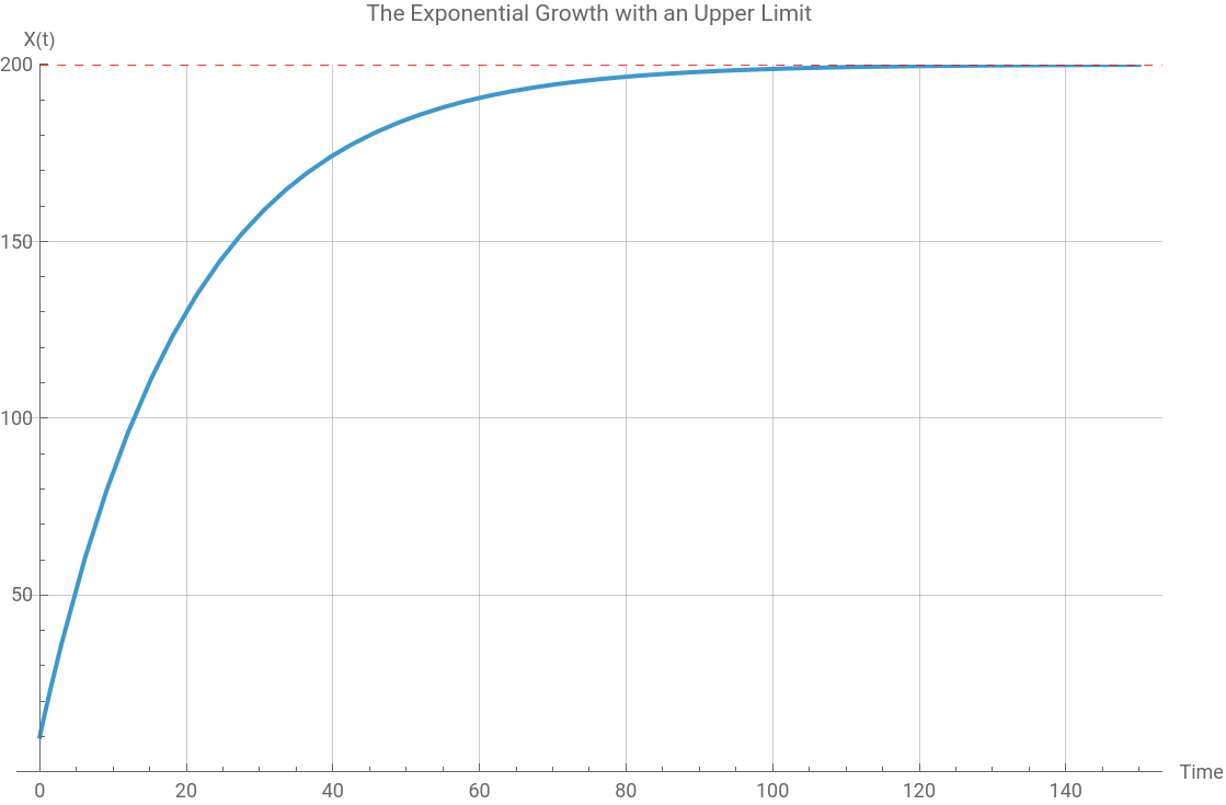
The population grow exponentially at first. But as it reaches a particular level, the carrying capacity of K = 200, its growth rate is slowing down.
The logistic growth pattern
The logistic growth pattern
Finally, let us suppose that the growth of population is not constant but changing as the size of population changes. We will assume that the relative rate of increase in population is approximately constant when the population is small, but it converges to zero as the population approaches its carrying capacity, K.
A special form of this assumption is expressed by the equation, (t) = r X(t)(1 - ). This equation tells us that when the population X(t) is small in relation to K, so that is close to zero, then (t) ≃ rX(t), which implies that X(t) grows exponentially. As X(t) becomes larger, however, the factor 1 - begins to influence the behavior of the exponential growth part of the differential equation.
X
X(t)
K
x(t)
K
X
x(t)
K
The solution to this differential equation is X(t) = where A = . This particular differential equation is called the logistic growth model or logistic function.
K
1+A
-rt
K-X0
X0
In[]:=
Clear[X,t,r,K,X0];DSolve[{X'[t]==rX[t](1-X[t]/K),X[0]==X0},X[t],t]
Out[]=
X[t]KX0
rt
K-X0+X0
rt
Using the same numerical examples, K = 200, X0 = 10 and r = 0.05, we can visualize this logistic function as follows:
In[]:=
Clear[X,t];K=200;r=0.05;X0=10;X[t_]:=KX0;
rt
K-X0+X0
rt
In[]:=
Plot[X[t],{t,0,150},PlotLabel->"The Logistic Growth",AxesLabel->{"Time","X(t)"},GridLinesAutomatic,PlotRange->{0,200},Epilog->{Dashed,Red,Line[{{0,K},{200,K}}],Text[Style["Carrying Capacity (K)",Red,12],{150,K},{0,-1}]}]
Out[]=
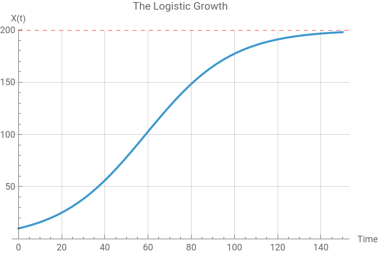
Notice that the shape (or the slope) of this function is changing over time: At the beginning, the exponential growth pattern is much stronger. But as time goes by the negative feedback comes into play, suppressing the initial exponential growth part of population. The second half of the growth pattern looks a lot more similar to the exponential growth with an upper limit.
Adam Smith’s capital stock growth model
Adam Smith’s capital stock growth model
Introduction
Introduction
As an example of the three growth patterns, let us reconstruct Adam Smith’s implied economic growth model. Among many powerful ideas in Smith’s Wealth of Nations, we want to focus on his incomplete but important analysis of the interaction between capital accumulation and the change in the demand for labor.
In the context of analysing the process and effect of the accumulation of the capital stock, Smith suggests that that the growth of the fixed capital stock tends to pull a greater number of workers whose labor is being used in the production process.
This idea is what our contemporary economists call ‘the relationship between the accumulation of capital stock and the corresponding change in the demand for labor.’ How can we build a model that captures the essence of Smith’s ideas? Where does Smith’s ideas fit into the three growth patterns?
The baseline model
The baseline model
The specification of variables and parameters
The specification of variables and parameters
Suppose that the size of population and labor force are temporarily fixed, and there is an average nominal wage rate prevailing in an industry.
Let us denote K(t) the productive capital stock used in Smith’s manufacture at time t, L(t) the demand for a unit of labor at time t, which is the same thing as the number of workers who are employed in the industry given the average working hour per period. Suppose that a is the net average rate of profit and b the average capital-labor ratio, both of which are assumed to be constant here.
The equations for the model
The equations for the model
If we further assume that the fixed capital stock in manufacture grows at a rate consistent with the average rate of profit, we can set the following differential equation for the growth of the capital stock:
This equation means that the change in the capital stock is a positive function of the existing capital stock (assuming a > 0). How fast the capital stock grows depends on the size of a, the net average industrial rate of profit.
Since we have introduced a constant capital-labor ratio, b, the change in the demand for labor is also written as:
The second equation means that the change in the demand for labor is a positive function of the capital stock. If the productive capital stock in manufacture grows, it will require a greater utilization of human labor, requiring that a greater number of workers be hired (given the average working hour per period) and put in the production process. The intensity of this labor demand is determined by the value of b (b > 0).
These two linear, first-order, homogenous, autonomous differential equations constitute an important baseline economic model that shows the relationship between the change in the fixed capital stock and the change in the demand for labor input.
The analytical solution of the model
The analytical solution of the model
Taking advantage of Mathematica’s computational power, we can find the following analytical solution:
The visualization of the solution with fixed parameters and initial values
The visualization of the solution with fixed parameters and initial values
To see the dynamic behavior of the solution of this differential equations model, let us assign the following arbitrary values to the parameters, a and b, and the initial condition, K0 and L0:
The interactive visualization of the solution with varying parameter values
The interactive visualization of the solution with varying parameter values
Suppose now that you want to create an interactive graph that shows the instantaneous change in the behavior of the solution curves with varying parameter values. We can use the following syntax for this purpose:
Concluding remark
Concluding remark
In this section, we have replicated Smith’s capital stock growth model assuming that (1) the growth rate of the capital stock is constant and (2) the demand for labor (or the capital-labor ratio) is also constant. With these two assumptions, we have seen that Smith’s implicit ideas about the economic growth process is one of the exponential growth models.
David Ricardo’s capital stock growth model
David Ricardo’s capital stock growth model
Introduction
Introduction
David Ricardo also provides his ideas about the capital stock growth process. Unlike Smith, however, Ricardo held a pessimistic view on the long-run consequence of the capital stock accumulation. He observes that the rapid accumulation of the capital stock brings about a higher demand for labor, which will increase nominal wages. The same process tends to induce a greater quantity of arable land to be cultivated as the number of employed workers demand greater amounts of food and necessaries.
The increase in the demand for agricultural land for food production and rising demand for labor/higher nominal wages, both of which are endogenously generated by the accumulation of the capital stock in the agricultural sector, soon becomes an obstacle that impedes a further accumulation of the capital stock in the same sector. From a mathematical point of view, Ricardo’s idea can be best described as the one of an exponential growth with an upper limit, which is different from Smith’s exponential growth model.
The baseline model
The baseline model
The specification of variables and parameters
The specification of variables and parameters
Let us denote K(t) the capital stock at time t, L(t) the demand for a unit of labor at time t, which is the same thing as the number of workers who are employed in the industry given the average working hour per period, and T(t) the fixed arable land for agricultural production. In this formulation, the arable land is fixed. Therefore, T(t) = T.
Suppose that a(t) is the net investment rate at time t and b(t) the average capital-labor ratio at time t, both of which are assumed to be constant. Finally, r(t) = r is the average rate of rent at time t in this economy.
The equations for the model
The equations for the model
The capital stock can grow with a fixed investment rate, a (a> 0), but there is an absolute limit beyond which it cannot grow any more. This upper limit is constrained by the quantity of arable land (T).
As before, we assume that there is a fixed capital-labor ratio, b (b>0). As the volume of the capital stock increases, there will be a greater demand for labor, whose exact quantity is determined by this ratio.
Ricardo himself did not specify how the labor force changes. Therefore, we can temporarily ignore the labor force growth variable and assume that the change in the demand for labor is a positive function of the growth of the capital stock even when it may be possible that the increase in the demand for labor is beyond the total labor force.
Finally, suppose that the need of cultivating land for agricultural production at time t, A(t), is subject to the change in the agricultural capital stock where r represents a speed of the capital stock accumulation.
The analytical and numerical solution with fixed parameters and initial values
The analytical and numerical solution with fixed parameters and initial values
The analytical solution to this system can be found by:
Suppose now we have the following arbitrary parameters and initial conditions of the three stocks:
The interactive visualization of the solution with varying parameter values
The interactive visualization of the solution with varying parameter values
Finally, let us create an interactive graph that shows the instantaneous change in the behavior of the solution curves with varying parameter values. For this simulation, we are focused on the capital accumulation and the utilization of land only:
Concluding remark
Concluding remark
Ricardo’s capital stock growth model is one of the exponential growth with the upper limit where this upper limit is governed by the total arable land available in the economy. As the accumulation of the capital stock in the agricultural sector proceeds, more land is being leased and cultivated, ultimately reaching its absolute limit. The economy enters what Ricardo called the long-run “stationary state.”
For our convenience, we have assumed that both the investment rate and the capital-labor ratio are constant in this simulation. If we introduce an income-distribution parameters and a theory of labor productivity change, we can relax these assumptions to make this baseline model more realistic. We can also modify the exponential growth pattern of the labor demand by introducing a certain labor force growth pattern that may constrain the growth of the demand for labor in the economy.
Conclusion
Conclusion
In this note, we learn how we can model the three representative growth patterns using Wolfram Mathematica. These are (1) the exponential growth without a limit, (2) the exponential growth with an upper limit, and (3) the logistic growth pattern. As an example of the first two growth patterns, we have reconstructed both Smith and Ricardo’s respective view about how the economy will grow over time. Smith’s optimistic vision of the economic growth and development in the early stage of capitalism is one of the exponential growth pattern, whereas Ricardo’s rather pessimistic view is the one that we call the exponential growth with an upper limit.
Reference
Reference
◼
Adam Smith, An Inquiry into the Causes and Nature of the Wealth of Nations (edited with an introduction and notes by Andrew Skinner), London: Penguin Books, 1999 [1776].
◼
David Ricardo, Principles of Political Economy and Taxation, Amherst and New York: Prometheus Books, 1996 [1817] (based upon the 3rd edition published in 1821).
◼
Paul Blanchard, Robert L. Devaney, and Glen R. Hall, Differential Equations, Cengage Learning, 2012 (4th edition), pp.4-12.
CITE THIS NOTEBOOK
CITE THIS NOTEBOOK
Introduction to dynamic economic models: economic growth and growth models
by Hee-Young Shin
Wolfram Community, STAFF PICKS, January 6, 2026
https://community.wolfram.com/groups/-/m/t/3602110
by Hee-Young Shin
Wolfram Community, STAFF PICKS, January 6, 2026
https://community.wolfram.com/groups/-/m/t/3602110