Uniquac Model for Pentanary Liquid - Phase Split
Authors: Siwar Labidi and Housam Binous
Uniquac Model for Pentanary Liquid - Phase Split
Authors: Siwar Labidi and Housam Binous
Authors: Siwar Labidi and Housam Binous
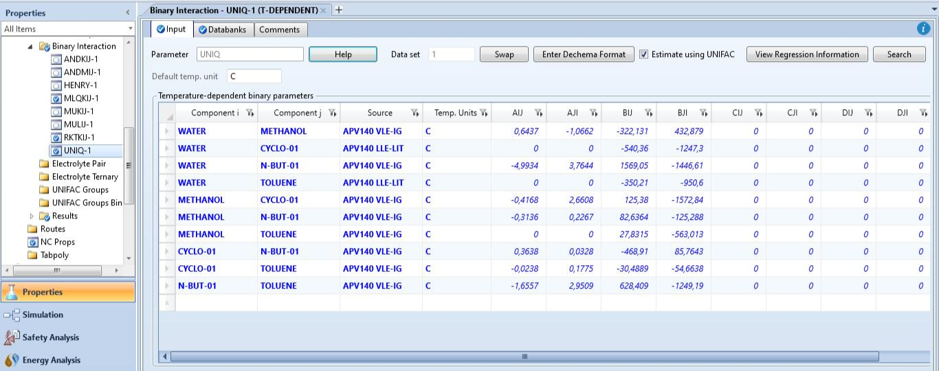
The code implements the UNIQUAC activity coefficient model for a five-component liquid-liquid equilibrium system consisting of Water, Methanol, Cyclohexane, n-Butanol, and Toluene at 25°C and atmospheric pressure. Pure component structural parameters r and q are taken from Sandler’s textbook, while the 10 asymmetric binary interaction parameters are sourced directly from the Aspen Plus UNIQ-1 databank and arranged into 5×5 A and B matrices.
The activity coefficients are computed via the standard UNIQUAC combinatorial and residual contributions, with the interaction energy expressed as τᵢⱼ = exp(Aᵢⱼ + Bᵢⱼ/T), where T is in Kelvin.
Phase stability is first confirmed using the Tangent Plane Distance criterion, where a global minimum of TPD = −0.3148 indicates the feed composition z = {0.30, 0.15, 0.25, 0.20, 0.10} is unstable and must split into two phases.
The equilibrium compositions are then found by simultaneously solving four iso-activity conditions, four Rachford-Rice composition equations, and the Rachford-Rice summation equation — nine equations in nine unknowns — using least-squares minimization. The result yields a water-rich phase (xᵅ) dominated by Water and n-Butanol, and an organic-rich phase (xᵝ) dominated by Cyclohexane and Toluene, with a phase-beta fraction of β = 0.3537.
Mathematica results show excellent agreement with their counterparts obtained using Aspen-Plus.
Based on the converged LLE solution:
Liquid Phase 1 (α — Aqueous-rich phase):
The first liquid phase is predominantly aqueous, with Water as the dominant component at a mole fraction of 0.4612, followed by n-Butanol at 0.2649 and Methanol at 0.2184. Cyclohexane and Toluene are nearly immiscible in this phase, appearing at very low mole fractions of 0.0329 and 0.0226 respectively. The presence of Methanol and n-Butanol in this phase reflects their partial miscibility with water due to their hydroxyl groups.
Liquid Phase 2 (β — Organic-rich phase):
The second liquid phase is organic-rich, dominated by Cyclohexane at 0.6466 and Toluene at 0.2413, which together account for over 85% of the phase composition. n-Butanol appears at 0.0815, acting as a bridging component between the aqueous and organic phases due to its amphiphilic nature. Methanol and Water are largely expelled from this phase, present only at trace levels of 0.0251 and 0.0055 respectively, consistent with their strong affinity for the aqueous phase.
Phase split fraction:
The organic phase (β) constitutes 35.37% of the total mixture, while the aqueous phase (α) accounts for the remaining 64.63%, reflecting the water-rich nature of the overall feed composition z = {0.30, 0.15, 0.25, 0.20, 0.10}.
In[]:=
(* 1=Water, 2=Methanol, 3=Cyclohexane, 4=n-Butanol, 5=Toluene *)
In[]:=
(*UNIQUACvolume(r)andsurfacearea(q)parameters*)(*Source:Sandler"Chemical Engineering Thermodynamics",App.D*)r={0.9200,1.4311,4.0464,3.4543,3.9228};q={1.40002,1.43203,3.24004,3.04805,2.9700};
In[]:=
(*UNIQUACBinaryInteractionParametersfromAspenPlus(UNIQ-1,T-Dependent)*)(*tau_ij=Exp[aij+bij/T]whereTisinKelvin*)params={{"WATER","METHANOL",0.6437,-1.0662,-322.131,432.879},{"WATER","CYCLO-01",0,0,-540.36,-1247.3},{"WATER","N-BUT-01",-4.9934,3.7644,1569.05,-1446.61},{"WATER","TOLUENE",0,0,-350.21,-950.6},{"METHANOL","CYCLO-01",-0.4168,2.6608,125.38,-1572.84},{"METHANOL","N-BUT-01",-0.3136,0.2267,82.6364,-125.288},{"METHANOL","TOLUENE",0,0,27.8315,-563.013},{"CYCLO-01","N-BUT-01",0.3638,0.0328,-468.91,85.7643},{"CYCLO-01","TOLUENE",-0.0238,0.1775,-30.4889,-54.6638},{"N-BUT-01","TOLUENE",-1.6557,2.9509,628.409,-1249.19}};(*tau_ijandtau_ji,TinKelvin*)tauIJ[aij_,bij_,T_]:=Exp[aij+bij/T]tauJI[aji_,bji_,T_]:=Exp[aji+bji/T](*Evaluatealltau_ijandtau_jiattemperatureTcinCelsius*)EvalTau[Tc_]:=Module[{TK=Tc+273.15},TableForm[Table[{params[[k,1]],params[[k,2]],N@tauIJ[params[[k,3]],params[[k,5]],TK],(*tau_ij*)N@tauJI[params[[k,4]],params[[k,6]],TK](*tau_ji*)},{k,1,Length[params]}],TableHeadings->{None,{"i","j","tau_ij","tau_ji"}}]]
In[]:=
params//TableForm
Out[]//TableForm=
WATER | METHANOL | 0.6437 | -1.0662 | -322.131 | 432.879 |
WATER | CYCLO-01 | 0 | 0 | -540.36 | -1247.3 |
WATER | N-BUT-01 | -4.9934 | 3.7644 | 1569.05 | -1446.61 |
WATER | TOLUENE | 0 | 0 | -350.21 | -950.6 |
METHANOL | CYCLO-01 | -0.4168 | 2.6608 | 125.38 | -1572.84 |
METHANOL | N-BUT-01 | -0.3136 | 0.2267 | 82.6364 | -125.288 |
METHANOL | TOLUENE | 0 | 0 | 27.8315 | -563.013 |
CYCLO-01 | N-BUT-01 | 0.3638 | 0.0328 | -468.91 | 85.7643 |
CYCLO-01 | TOLUENE | -0.0238 | 0.1775 | -30.4889 | -54.6638 |
N-BUT-01 | TOLUENE | -1.6557 | 2.9509 | 628.409 | -1249.19 |
In[]:=
In[]:=
A={{0,0.6437,0,-4.9934,0},{-1.0662,0,-0.4168,-0.3136,0},{0,2.6608,0,0.3638,-0.0238},{3.7644,0.2267,0.0328,0,-1.6557},{0,0,0.1775,2.9509,0}};
In[]:=
Dimensions[A]
Out[]=
{5,5}
In[]:=
B={{0,-322.131,-540.36,1569.05,-350.21},{432.879,0,125.38,82.6364,27.8315},{-1247.3,-1572.84,0,-468.91,-30.4889},{-1446.61,-125.288,85.7643,0,628.409},{-950.6,-563.013,-54.6638,-1249.19,0}};
In[]:=
Dimensions[B]
Out[]=
{5,5}
In[]:=
T=298.15;
In[]:=
(*Example:evaluateat25C*)EvalTau[25]
Out[]//TableForm=
i | j | tau_ij | tau_ji |
WATER | METHANOL | 0.646144 | 1.47062 |
WATER | CYCLO-01 | 0.163266 | 0.0152456 |
WATER | N-BUT-01 | 1.30894 | 0.33704 |
WATER | TOLUENE | 0.308939 | 0.0412408 |
METHANOL | CYCLO-01 | 1.00373 | 0.0732021 |
METHANOL | N-BUT-01 | 0.96422 | 0.824055 |
METHANOL | TOLUENE | 1.09784 | 0.151321 |
CYCLO-01 | N-BUT-01 | 0.298516 | 1.37775 |
CYCLO-01 | TOLUENE | 0.881562 | 0.994174 |
N-BUT-01 | TOLUENE | 1.57144 | 0.289702 |
In[]:=
nc=5;
In[]:=
Table[Exp[A[[i,j]]+B[[i,j]]/T],{i,1,nc},{j,1,nc}]//TableForm
Out[]//TableForm=
1. | 0.646144 | 0.163266 | 1.30894 | 0.308939 |
1.47062 | 1. | 1.00373 | 0.96422 | 1.09784 |
0.0152456 | 0.0732021 | 1. | 0.298516 | 0.881562 |
0.33704 | 0.824055 | 1.37775 | 1. | 1.57144 |
0.0412408 | 0.151321 | 0.994174 | 0.289702 | 1. |
In[]:=
(*UNIQUACACTIVITYCOEFFICIENTFUNCTION*)UNIQUACgamma[x_List]:=Module[{nc,phi,theta,tau,lnGammaComb,lnGammaRes,lnGamma,z0=10,l,S,sumXL},nc=Length[x];(*Coordinationnumberz0=10*)l=Table[(z0/2)(r[[i]]-q[[i]])-(r[[i]]-1),{i,1,nc}];(*Segment&surfacefractions*)phi=(r*x)/(r.x);theta=(q*x)/(q.x);(*UNIQUACtaumatrix*)tau=Table[Exp[A[[i,j]]+B[[i,j]]/T],{i,1,nc},{j,1,nc}];(*---Combinatorialpart---*)sumXL=Sum[x[[i]]l[[i]],{i,1,nc}];lnGammaComb=Table[Log[phi[[i]]/x[[i]]]+(z0/2)q[[i]]Log[theta[[i]]/phi[[i]]]+l[[i]]-(phi[[i]]/x[[i]])sumXL,{i,1,nc}];(*---Residualpart---*)S=Table[Sum[theta[[j]]tau[[j,i]],{j,1,nc}],{i,1,nc}];lnGammaRes=Table[q[[i]](1-Log[S[[i]]]-Sum[theta[[k]]tau[[i,k]]/S[[k]],{k,1,nc}]),{i,1,nc}];lnGamma=lnGammaComb+lnGammaRes;Exp[lnGamma]];
In[]:=
(*Feedmolefractions*)z={0.30,0.15,0.25,0.20,0.10}
Out[]=
{0.3,0.15,0.25,0.2,0.1}
In[]:=
T=298.15;(*Temperature25°C*)
In[]:=
gammaZ=UNIQUACgamma[z]
Out[]=
{4.30263,0.999834,4.37602,0.848281,3.50718}
In[]:=
Clear[TPD];TPD[w1_?NumericQ,w2_?NumericQ,w3_?NumericQ,w4_?NumericQ]:=Module[{w5,w,gammaW},w5=1-w1-w2-w3-w4;If[w1<=0||w2<=0||w3<=0||w4<=0||w5<=0,Return[10^10]];w={w1,w2,w3,w4,w5};gammaW=UNIQUACgamma[w];Sum[w[[i]]*(Log[w[[i]]*gammaW[[i]]]-Log[z[[i]]*gammaZ[[i]]]),{i,1,5}]]sol=NMinimize[{TPD[w1,w2,w3,w4],w1>=10^-6,w2>=10^-6,w3>=10^-6,w4>=10^-6,1-w1-w2-w3-w4>=10^-6},{w1,w2,w3,w4},Method->{"DifferentialEvolution"}];TPDmin=sol[[1]];Print[" TPDmin = ",NumberForm[TPDmin,{12,8}]]