Overview: How This Notebook Is Set
Overview: How This Notebook Is Set
This notebook explores whether a quantum particle can remain bound by its own gravitational field. This phenomenon is described by the Schrödinger–Newton equation, in which the particle interacts with the gravitational field generated by its own mass. Throughout this notebook, we refer to this gravitational self-interaction simply as self-gravity.
Quantum mechanics predicts that a localized wavepacket naturally spreads over time. In contrast, the Schrödinger–Newton equation introduces self-gravity, which pulls the particle’s mass inward. As a result, the particle experiences two competing effects: quantum dispersion tends to spread the wavepacket, while self-gravity tends to localize it. If these effects exactly balance, the particle can form a stable, localized wavepacket known as a gravitational soliton.
The goal of this notebook is to compute the gravitational soliton. We begin with a simple energy estimate, then reduce the three-dimensional problem to a one-dimensional radial equation. Next, we solve the coupled Schrödinger–Newton equations iteratively, eliminate the effects of the artificial boundary introduced by the finite computational domain, and finally verify the solution using an exact virial relation.
The main steps in the notebook are:
◼
explain the idea in words,
◼
compute and verify it in the Wolfram Language,
◼
then interpret what the output means.
Some code cells are naturally technical, especially the finite-element solver. My suggestion is to first read what the cell is meant to do and what its output means. After that, you can return to the details of the input code. You should also change the box size, mesh size, and initial guess to see how robust the calculation is.
You should be comfortable with the time-independent Schrödinger equation, spherical symmetry, and the idea of an eigenvalue problem. It helps if you have used and , but the important steps are explained as we go. Additionally, I highly recommend if you read our doc page on Schrodinger-Newton equation.
Let's start!
Quantum Spreading against Self-Gravity
Quantum Spreading against Self-Gravity
Take a free quantum particle and put it in a small region. It will not stay there. The wavefunction spreads, and the more tightly we localize it at the beginning, the faster it tends to spread.
Generate numerical solution for evolution of a free particle using Schrodinger equation:
In[]:=
ℋ=SchrodingerPDEComponent[{Ψ[t,x],t,{x}},<|"Mass"->1,"ReducedPlanckConstant"->1,"SchrodingerPotential"->0|>];solution1=NDSolveValue{ℋ==0,Ψ[0,x]==Exp[-(x^2)]},Ψ,{t,0,3},{x,-20,20},Method->;solution2=NDSolveValue{ℋ==0,Ψ[0,x]==Exp[-(x^2)/8]},Ψ,{t,0,3},{x,-20,20},Method->;
Visualize the evolution:
In[]:=
AnimatePlotEvaluate[{,}],{x,-10,10},,{{t,0.5},0,3,0.1},
2
Abs[solution1[t,x]]
2
Abs[solution2[t,x]]
Out[]=
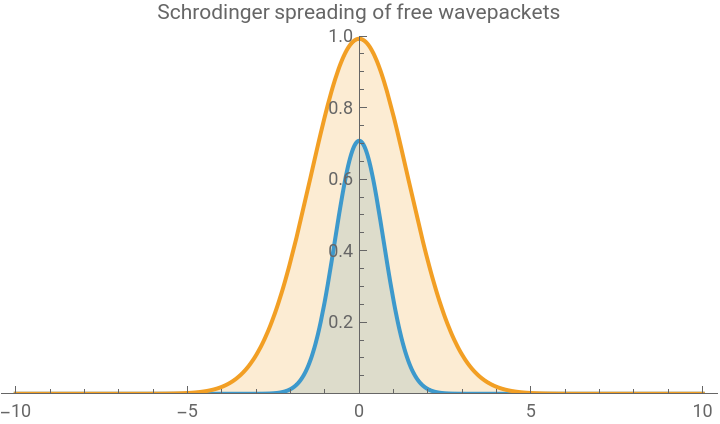
As expected, the more localized blue wavepacket spreads more rapidly than the less localized one.
Now let the particle feel the gravitational field produced by its own mass density, . Then the particle is both the source of the field and the object moving in that field. This is the idea behind the Schrödinger-Newton equation. Note the unit of is the same as mass density (in SI, ).
m
2
ψ |
m
2
ψ |
kg
3
m
In simple words:
◼
The standard quantum dynamical equation implies that the wavefunction is pushed outward by spreading it,
◼
gravity pulls the wavefunction inward,
◼
a soliton appears when the two effects balance.
Note that a soliton is a waveform that moves but does not change it’s shape through, for example, diffusion.
The Schrödinger-Newton equation is a simple model to explain the appearance of a soliton wave of a particle; it is not a theory of quantum gravity. It is also not a collapse model. The Schrödinger-Newton equation is a deterministic equation and treats the gravitational field as classical, while the matter is described by a quantum wavefunction. In that sense it is a mean-field approximation where the gravitational field is sourced by the average mass density of the quantum state.
As a first step, we can estimate the size of the bound state. Suppose the particle is confined to a region of size . The kinetic energy cost of squeezing the wavefunction scales like /(m). In contrast, the gravitational self-interaction is attractive and scales like . So the total energy has the rough form
ℓ
2
ℏ
2
ℓ
-G/ℓ
2
m
Let’s minimize the energy estimate as a function of the assumed size :
ℓ
In[]:=
Solve[D[ℏ^2/(mℓ^2)-Gm^2/ℓ,ℓ]==0,ℓ]
Out[]=
ℓ
2
2
ℏ
G
3
m
The factor of 2 is not important for setting the scale, so we define the natural scaled length of the problem as
This estimate already tells us the main physical picture. If the packet is much wider than , gravity pulls it inward. If it is much narrower than , kinetic energy pushes it outward. Near , the two effects can balance.
ℓ
★
ℓ
★
ℓ
★
The strong mass dependence is also important: scales like . For an electron, because its mass is extremely small, this length is enormously large (), so gravity is far too weak to produce any meaningful self-binding. The effect is therefore completely negligible. For much heavier objects, such as massive molecules, nanoparticles, or mesoscopic objects, the balance can become more relevant. For example, for a nanoparticle of the mass amu, the scaled length is of the order m.
ℓ
★
1/
3
m
~m
32
10
10
10
-7
10
From Three Dimensions to One Dimension
From Three Dimensions to One Dimension
The full Schrödinger-Newton equation is system of two coupled equations. The wavefunction moves in the gravitational potential , and the potential is created by the mass density of :
ψ
Φ
Φ
ψ
The equations are coupled. To find , we need . To find , we need .
ψ
Φ
Φ
ψ
We make two simplifications.
First, we choose scaled units. Setting , and measuring length in units of , also sets . After this rescaling, there are no free physical constants in the now dimensionless equation. The ground-state energy becomes a pure number. This number has no closed form; the value found numerically in the literature, by Moroz, Penrose and Tod [1], is , and reproducing it from scratch is the goal of this notebook.
ℏ=m=1
ℓ
★
G=1
-0.163
Second, we assume spherical symmetry and thus a ground state has no preferred direction, so it depends only on the radius . We write a stationary state as
r
where is a real-valued radial function.
f(r)
Define a new radial function:
Now plugging into Schrödinger-Newton equation together with above change of variables and scaled units, the equations become:
ψ(r,t)=f(r)
-iEt
e
The equation for is now an ordinary one-dimensional Schrödinger eigenvalue problem. It has the same form as a particle moving on a straight line in the potential .
u
Φ(r)
There are two related but different quantities to keep in mind:
◼
2
f(r) |
◼
u=4π
2
(r)
2
r
2
f(r) |
The full three-dimensional normalization in Cartesian coordinates, i.e. (no integration bound, since the particle can be free, for example), becomes the one-dimensional condition in the -direction in spherical coordinates:
∫
X=1
2
ψ |
3
d
r
In Version 15.0 the WL cannot numerically solve equations over an infinite interval , so we solve on a finite interval . The number is the box radius. It is not physical. It is a numerical boundary that we will later remove by extrapolation.
0≤r<∞
0≤r≤R
R
The boundary conditions are:
◼
u(0)=0
f(r)
◼
u(R)=0
◼
Φ(R)=0
◼
R
∫
0
2
(r)
With no condition specified explicitly at , it means we have a Neumann zero boundary condition, i.e. .
r=0
Φ'(0)=0
One fact about will matter later. Far from the cloud where the particle is localized, the whole mass looks like a unit point mass. Therefore, at large enough , the potential approaches:
Φ
r
This far-out part, the tail of the potential, decays slowly, as a power of rather than exponentially, so it never quite reaches zero at any finite radius; this is what “long-range” means, and it is the same slow falloff as the Coulomb field. That slow decay is exactly what makes a finite box costly: forcing at a finite radius, we shift the potential upward by about . That creates a leading energy error proportional to . Later we will see this directly in the data.
r
Φ(R)=0
1/R
1/R
The Self-Consistent Loop
The Self-Consistent Loop
Because and determine each other, we solve them by iteration.
u
Φ
The idea is simple:
1- Guess a wavefunction .
2- Solve Newton’s equation to get the potential made by that .
3- Solve Schrödinger’s equation to get the ground state in that potential.
4- Repeat until the energy stops changing.
u
2- Solve Newton’s equation to get the potential
Φ
u
3- Solve Schrödinger’s equation to get the ground state in that potential.
4- Repeat until the energy stops changing.
This is called a self-consistent calculation because the final wavefunction must create the same potential that binds it.
Load the finite-element tools:
In[]:=
Needs["NDSolve`FEM`"]
Build the left-hand side of the Newton equation:
In[]:=
newtonOp=Laplacian[Φ[r],{r,θ,φ},"Spherical"]
Out[]=
2[r]
′
Φ
r
′′
Φ
The output is (r)+(2/r)(r), exactly the radial Newton operator we need.
″
Φ
′
Φ
Build the Schrödinger operator:
In[]:=
hamiltonianOp=SchrodingerPDEComponent[{u[r],{r}},<|"ReducedPlanckConstant"->1,"SchrodingerPotential"->Φ[r]|>]
Out[]=
u[r]Φ[r]+·-.u[r]
∇
{r}
1
2
∇
{r}
This gives the operator
Now we need a small helper for choosing the correct eigenstate. does not automatically return the most negative eigenvalue in the way we need. The ground state is the lowest energy state, so we sort the eigenvalues by their real part and take the first one.
NDEigensystem
Define a function that sorts eigenpairs by eigenvalue:
In[]:=
sortStates[s_]:=SortBy[Transpose[s],Re]//Transpose
The tiny imaginary parts that sometimes appear are numerical roundoff from the Arnoldi method used by . The operator is self-adjoint, so the physical eigenvalues are real.
NDEigensystem
Define the Newton solver. Given a wavefunction and a mesh, it returns the gravitational potential created by that wavefunction:
In[]:=
solveNewton[uFunc_,mesh_]:=NDSolveValue[{newtonOp==uFunc^2/r^2,DirichletCondition[Φ[r]==0,r==mesh["Bounds"][[1,2]]]},Φ,{r}∈mesh]
Define the Schrödinger solver. Given a potential and a mesh, it returns the lowest bound state:
Let’s elaborate on options we used above. Arnoldi is a variational method that finds the best eigensystem inside a small, properly chosen subspace. BasisSize is related to the dimension of that working subspace: how many independent trial directions the solver keeps before it restarts. With MaxIterations, we tell the solver that how long it may keep refining the subspace before giving up. An iterative solver naturally finds the eigenvalues closest to a chosen reference energy, and the default reference is zero. The Shift option move the reference far below the self-interaction gravity potential; the solver then returns the bound states, though not sorted, which is why the code sorts afterwards and asks for three states instead of one. The computed wavefunction is not a formula; it is a table of numbers on the mesh as a smooth function that is meaningful only inside the box. By default, evaluating it outside returns “undefined” and prints a complaint. The Interpolation option that we set, respects the fact that an approximation has a finite domain of validity, while it prevents edges from injecting undefined values.
Compute the norm:
Verify that this choice gives norm one:
Now assemble the full solver. It builds a mesh, starts from the Gaussian guess, alternates between the Newton and Schrödinger solvers, and stores the energy at every iteration:
Removing the Finite Box
Removing the Finite Box
Solve the self-consistent problem at six box radii:
Tabulate the final energy and the iteration count:
The fit gives
Visualize the energies approaching the infinite-box value:
Shifting each energy by its own box correction collapses the curve onto a horizontal line as shown below:
Reading the Soliton
Reading the Soliton
In this section, we look at the first three solitons and check how they behave.
Extract the reduced wavefunction, self-gravity potential, and the converged energy for the first three solitons:
Solve DEs:
A Consistency Check: The Virial Identity
A Consistency Check: The Virial Identity
A good numerical solution should satisfy a relation that was not built into the solver. Here that relation is the virial identity. In other words, this section is a sanity check of what we have computed.
Let the total energy functional be
where
is the kinetic energy, and
Now rescale the wavefunction by
Check the kinetic scaling with a concrete function:
So we have two equations:
The result is
Correct the eigenvalue by removing this shift:
The same argument predicts that
Compare the measured value with the prediction:
So the virial error is almost exactly the finite-box boundary shift. After removing that shift, the virial relation is recovered:
Where This Leaves Us
Where This Leaves Us
Let us summarize what we built.
We started from the physical competition between quantum spreading and gravitational attraction. A simple energy estimate gave the natural size
Then we used spherical symmetry and the substitution
to reduce the three-dimensional Schrödinger-Newton system to a one-dimensional radial problem. We solved that problem by a self-consistent finite-element loop: wavefunction gives potential, potential gives wavefunction, and the loop continues until the energy settles.
The most important computed facts are:
A natural next step is the time-dependent problem: evolve a general wavepacket under the full Schrödinger-Newton equation and compare it with the soliton, which holds its shape, and explore the stability of solitons to some perturbation.
Acknowledgment
Acknowledgment
This tutorial owes a great deal to colleagues at Wolfram Research, who read earlier drafts and pushed back on them. I am grateful for it.
References
References
2
.Harrison, R., Moroz, I. & Tod, K. P. (2003). A numerical study of the Schrödinger-Newton equations. Nonlinearity 16, 101-122 (arXiv:math-ph/0208045, math-ph/0208046). Linear stability of the ground state and instability of the excited states; the first twenty eigenvalues and the virial relations.
3
.Bernstein, D. H., Giladi, E. & Jones, K. R. W. (1998). Eigenstates of the gravitational Schrödinger equation. Mod. Phys. Lett. A 13, 2327.
4
.Bahrami, M., Großardt, A., Donadi, S. & Bassi, A. (2014). The Schrödinger-Newton equation and its foundations. New J. Phys. 16, 115007. doi:10.1088/1367-2630/16/11/115007. Derives the one-particle equation as a mean-field self-gravitation and separates it carefully from gravitationally induced collapse models.
CITE THIS NOTEBOOK
CITE THIS NOTEBOOK
Gravitational soliton ground state: finite-element extrapolation and virial verification
by Mads Bahrami
Wolfram Community, STAFF PICKS, July 2, 2026
https://community.wolfram.com/groups/-/m/t/3743040
by Mads Bahrami
Wolfram Community, STAFF PICKS, July 2, 2026
https://community.wolfram.com/groups/-/m/t/3743040