Consider a binary mixture with constant relative volatility, , subject to a batch rectification. Initially the binary mixture in the still is equimolar. The rectifying section has stages. A very large reflux ratio is chosen so that the Fenske equation is valid (see Ref. 1).
α
n
In such a case, the still and distillate compositions, versus the warped time, are given by (see Ref. 2) :=- where ξ is a warped time ( ). and =.
d
x
B
dξ
x
B
N+1
α
x
B
1+(-1)
N+1
α
x
B
0≤ξ≤1.6
x
D
N+1
α
x
B
1+(-1)
N+1
α
x
B
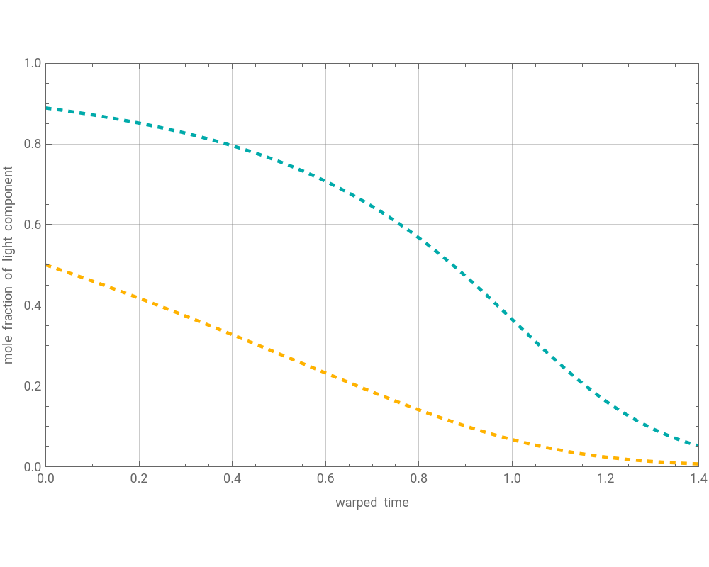
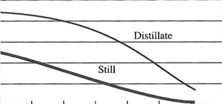
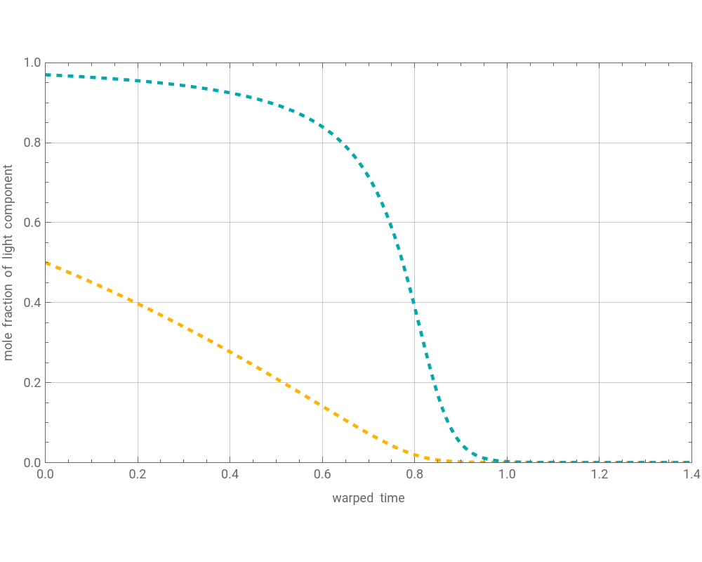
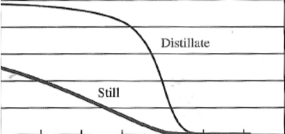
With this model, adding stages or increasing the relative volatility will produce the same effect. We display the mole fraction of the light component in the still (orange curve) and the distillate (blue curve) versus warped time. Adding more stages to the rectifying section (illustration 3) or increasing (illustration 4) will lead to a much more sharply defined variation in the distillate composition. We compare our results with their counterparts given in Fig. 9.2 of Ref. 2.
α
Illustration 1 : n=2 stages and α=2
In[]:=
α=2;(*relativevolatility*)
In[]:=
n=2;(*numberofstages*)
In[]:=
sol=NDSolveD[xB[ξ],{ξ,1}]xB[ξ]-xB[ξ],xB[0]0.5,{xB[ξ]},{ξ,0,1.6};
n+1
α
1+(-1)xB[ξ]
n+1
α
In[]:=
plt1=Plot[xB[ξ]/.sol,{ξ,0,1.6},FrameTrue,PlotRange{{0,1.4},{0.0,1}},FrameLabel{"warped time","mole fraction of light component"},PlotStyle{Thickness[.005],Dashed,RGBColor[1,0.7,0]},ImageSize{500,400},AxesOrigin{0,0.}];
In[]:=
plt2=PlotxB[ξ]/.sol,{ξ,0,1.6},FrameTrue,PlotRange{{0,1.4},{0.0,1}},AxesOrigin->{0,0},FrameLabel{"warped time","mole fraction of light component"},PlotStyle{Thickness[.005],Dashed,Darker@Cyan},ImageSize{500,400};
n+1
α
1+(-1)xB[ξ]
n+1
α
In[]:=
Show[plt1,plt2,GridLines->Automatic]
Out[]=
In[]:=
IMG=
;
In[]:=
Show[plt1,plt2,Prolog{Raster[ImageData[IMG,DataReversedTrue],{Scaled[{0.00,0.00}],Scaled[{1,1}]}]}]
Out[]=
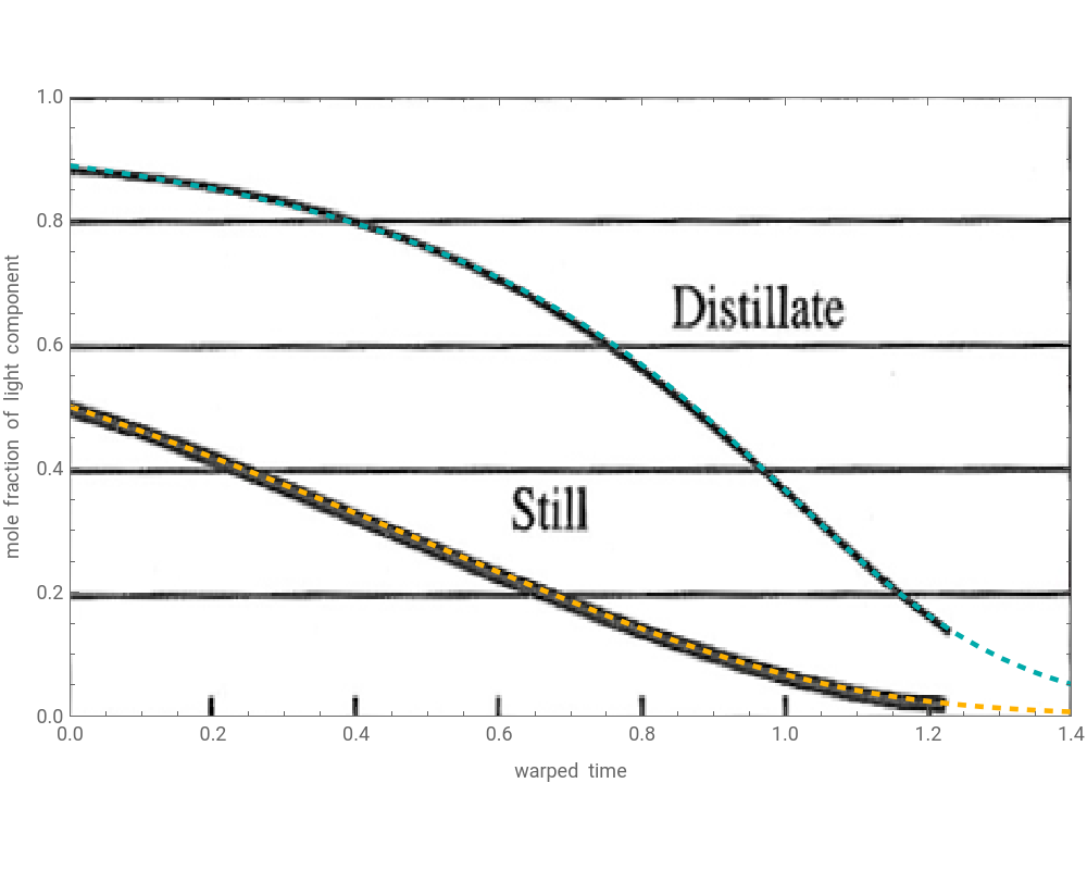
Illustration 2 : 4 stages and α=2
In[]:=
α=2;(*relativevolatility*)
In[]:=
n=4;(*numberofstages*)
In[]:=
sol=NDSolveD[xB[ξ],{ξ,1}]xB[ξ]-xB[ξ],xB[0]0.5,{xB[ξ]},{ξ,0,1.6};
n+1
α
1+(-1)xB[ξ]
n+1
α
In[]:=
plt1=Plot[xB[ξ]/.sol,{ξ,0,1.6},FrameTrue,PlotRange{{0,1.4},{0.0,1}},FrameLabel{"warped time","mole fraction of light component"},PlotStyle{Thickness[.005],Dashed,RGBColor[1,0.7,0]},ImageSize{500,400},AxesOrigin{0,0.}];
In[]:=
plt2=PlotxB[ξ]/.sol,{ξ,0,1.6},FrameTrue,PlotRange{{0,1.4},{0.0,1}},AxesOrigin->{0,0},FrameLabel{"warped time","mole fraction of light component"},PlotStyle{Thickness[.005],Dashed,Darker@Cyan},ImageSize{500,400};
n+1
α
1+(-1)xB[ξ]
n+1
α
In[]:=
Show[plt1,plt2,GridLines->Automatic]
Out[]=
In[]:=
IMG=
;
In[]:=
Show[plt1,plt2,Prolog{Raster[ImageData[IMG,DataReversedTrue],{Scaled[{0.00,0.00}],Scaled[{1,1}]}]}]
Out[]=
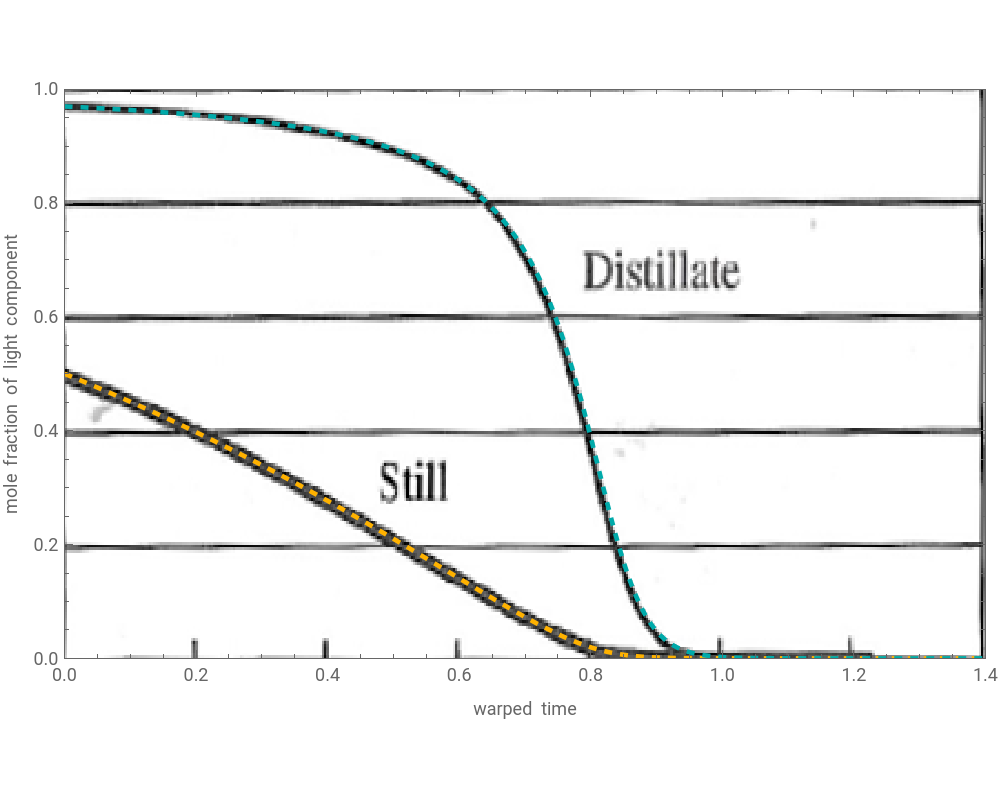
Illustration 3: n=8 stages and α=2
Here, a desirable situation occurs where there is a cut or a distillation fraction. Indeed, the distillate is quite pure for a period of time, then drops sharply when the light component is depleted in the still.
Here, a desirable situation occurs where there is a cut or a distillation fraction. Indeed, the distillate is quite pure for a period of time, then drops sharply when the light component is depleted in the still.
In[]:=
α=2;(*relativevolatility*)
In[]:=
n=8;(*numberofstages*)
In[]:=
sol=NDSolveD[xB[ξ],{ξ,1}]xB[ξ]-xB[ξ],xB[0]0.5,{xB[ξ]},{ξ,0,1.6};
n+1
α
1+(-1)xB[ξ]
n+1
α
In[]:=
plt1=Plot[xB[ξ]/.sol,{ξ,0,1.6},FrameTrue,PlotRange{{0,1.4},{0.0,1}},FrameLabel{"warped time","mole fraction of light component"},PlotStyle{Thickness[.005],Dashed,RGBColor[1,0.7,0]},ImageSize{500,400},AxesOrigin{0,0.}];
In[]:=
plt2=PlotxB[ξ]/.sol,{ξ,0,1.6},FrameTrue,PlotRange{{0,1.4},{0.0,1}},AxesOrigin->{0,0},FrameLabel{"warped time","mole fraction of light component"},PlotStyle{Thickness[.005],Dashed,Darker@Cyan},ImageSize{500,400};
n+1
α
1+(-1)xB[ξ]
n+1
α
In[]:=
Show[plt1,plt2,GridLines->Automatic]
Out[]=
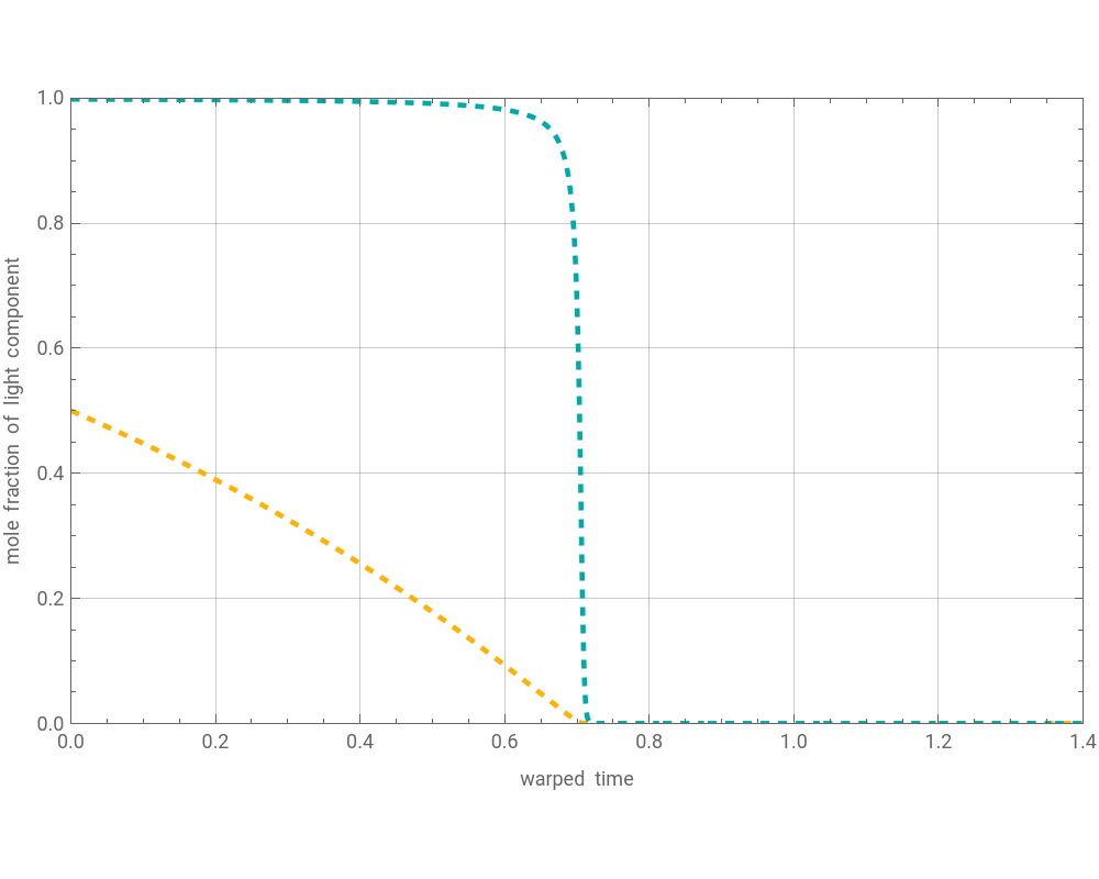
Illustration 4: n=4 stages and α=3.5
Here, a desirable situation also occurs where there is a cut or a distillation fraction. Indeed, the distillate is quite pure for a period of time, then drops sharply when the light component is depleted in the still.
Here, a desirable situation also occurs where there is a cut or a distillation fraction. Indeed, the distillate is quite pure for a period of time, then drops sharply when the light component is depleted in the still.
References
References
◼
[1] M.R. Fenske, Fractionation of Straight-Run Pennsylvania Gasoline, Ind.Eng. Chem., 24(5), pp. 482-485, 1932.
◼
[2] M. F. Doherty and M. F. Malone, Conceptual Design of Distillation Systems, Boston: McGraw-Hill, 2001.
CITE THIS NOTEBOOK
CITE THIS NOTEBOOK
Distillate and Still Compositions for Batch Rectification of a Binary Mixture at a Very Large Reflux
by Housam Binous and Ahmed Bellagi
Wolfram Community, STAFF PICKS, February 2, 2024
https://community.wolfram.com/groups/-/m/t/3114955
by Housam Binous and Ahmed Bellagi
Wolfram Community, STAFF PICKS, February 2, 2024
https://community.wolfram.com/groups/-/m/t/3114955