In a post in 2021 describing the Ruliad, Stephen Wolfram introduced the concept of the multiplicad, describing it “a rulial multiway system based on integers”. I examined the multiplicad and used my own restrictions to explore its properties. By calculating the Shapley values of each of the generators of a given multiplicad, we are able to quantitatively measure how much they impact the resulting structure.
Intro to the Multiplicad
Intro to the Multiplicad
What is it?
What is it?
The multiplicad is a sub-space of the Ruliad in which the computational pathways are limited to multiplication by natural numbers. Starting with a single node corresponding to the number 1, we multiply it by every natural number. Then, we multiply every subsequent product node by every natural number. As this process continues, we create edges between the nodes to notate that one is reached by multiplication from the other.
Out[]=
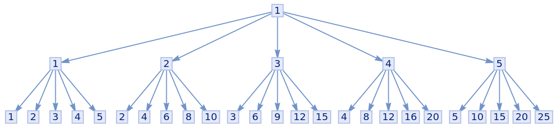
After the first iteration, every point has been reached as every natural number is a generator. After the second iteration, every edge connecting any two points is generated. The multiplicad grows infinitely larger each iteration, yet subsequent iterations simply regenerate information which already exists in the graph.
How do we use it?
How do we use it?
One interesting property of the multiplicad is that is has fractal qualities. Since every number is multiplied by every natural number including one, there are infinite appearances of every number. Most notably, by following the left side of each branch you repeat the same value over and over. Thus, creating the same branches over and over. However, when examining other properties of the multiplicad, it is often for convenient to deduplicate the graph: restrict each number to only appearing once in the entire graph. Furthermore, since including 1 as a generator of the multiplicad can only produce a number which is already present, it is more convenient to discard it as a generator entirely. Following these principles, the graph above could be shown like this.
Out[]=
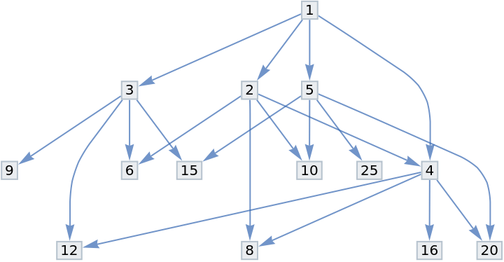
Every path in the first graph is still present in this version, except that they only appear once. This makes the underlying structure much more visible and eliminates redundant information.
Limiting Cases
Limiting Cases
Since the multiplicad uses all natural numbers as generators, to find specific properties, it is necessary to in some way limit it. We can do this in several ways. I explored limiting it by restricting the amount of generators we consider to always be a finite subset of the natural numbers to force the multiplicad to grow finitely fast. Additionally, by either setting a maximum value for which generated values that are greater than the max are not included or by calculating the product of each generator and node mod some number. Both ways ensure that the multiplicad can not to be infinitely large.
Properties
Properties
All properties
All properties
The graph we saw early shows what happens after only two iterations with the given generators, but if we iterate another time, we get this graph.
Out[]=
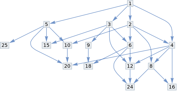
Any more than three iterations results in the same exact graph as this one. That is because these conditions correspond with equilibrium value of 3: the amount of iterations necessary before the resulting graph is identical to the one that would be produced with the same conditions and an additional iteration. Some other interesting properties of a multiplicad include the percentage of values less than the maximum value which are nodes in the graph, the number of nodes which have no subsequent nodes, the shortest path to the last node, and more.
Modular
Modular
If we substitute the above parameters into the modular version of the function, we get the graph below which requires 6 iterations before completion and is significantly more complicated.
Out[]=
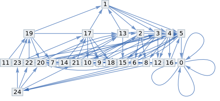
As shown in this graph, one of the properties unique to the modular version is that 0 can be generated. When a node and a generator multiply to the exact value of the mod being used, a zero is generated which gains as many recursive edges as there are generators on the next iteration.
Adding Generators
Adding Generators
Let’s consider a multiplicad with a single generator 2, and a max value of 30. This multiplicad requires 4 iterations before it reaches equilibrium. However, if we add generators 3 and 4, then it only takes 3 iterations. As we continue to add more and more generators until we reach the max value 30, we create the graph below.
Out[]=
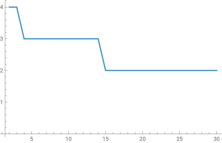
In all of these such graphs, it is always true that by the halfway point, the last drop in iteration from 3 to 2 occurs. On occasion it will happen before the halfway point, but since, at the halfway point, the first iteration generates all numbers from 2 to the halfway point, it is impossible for the next iteration not to generate all possible edges from each number to any other given number.
Alternatively, if instead of progressively adding each natural number as a generator, we can only consider the primes. Following the same pattern as in the graph above except only adding prime generators when we reach that number we get this graph.
Alternatively, if instead of progressively adding each natural number as a generator, we can only consider the primes. Following the same pattern as in the graph above except only adding prime generators when we reach that number we get this graph.
Out[]=
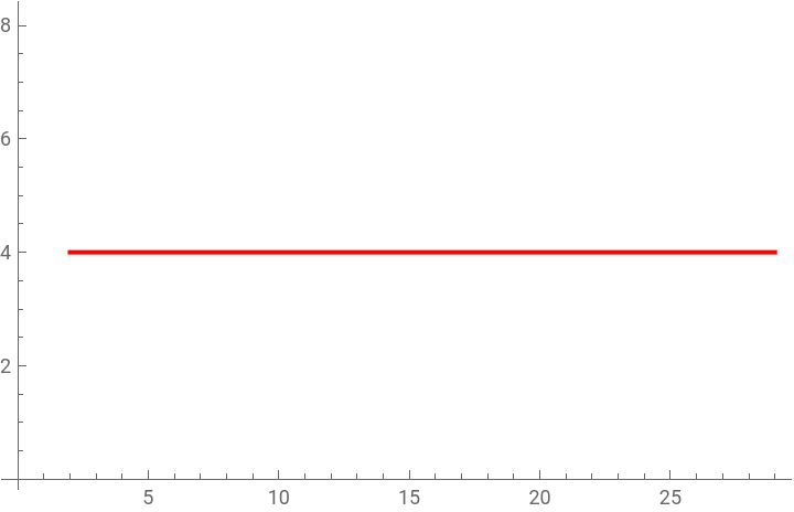
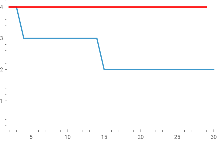
Regardless of how many prime numbers are added in a generators, the result is the same. This also happens if we consider coprime numbers. In these instances, the smallest generator will always take n iterations to reach equilibrium. The following generators, being larger than that one, can take at most n iterations. Thus, even if the other generators have finished generated everything they can, it will still always take n iterations. The reason that we don’t see this happen in the first example is because the smallest number is no relatively prime to the rest of them. Thus, the number of iterations until the smallest prime stops generating new edges is not independent from the rest of the generators.
By overlaying the two graphs, for all generators and only prime generators, you can visualize the effect that each non-relatively prime generator contributes.
By overlaying the two graphs, for all generators and only prime generators, you can visualize the effect that each non-relatively prime generator contributes.
Out[]=
Modular
Modular
The corresponding modular equivalents to these graphs are not so simple. The modular looping means that the graphs are not limited to be weakly decreasing. If we take the parameters for the graph representing all numbers, including the non-primes, and limit the multiplicad by modular loop rather than by a maximum, then we see a substantially different graph.
Out[]=
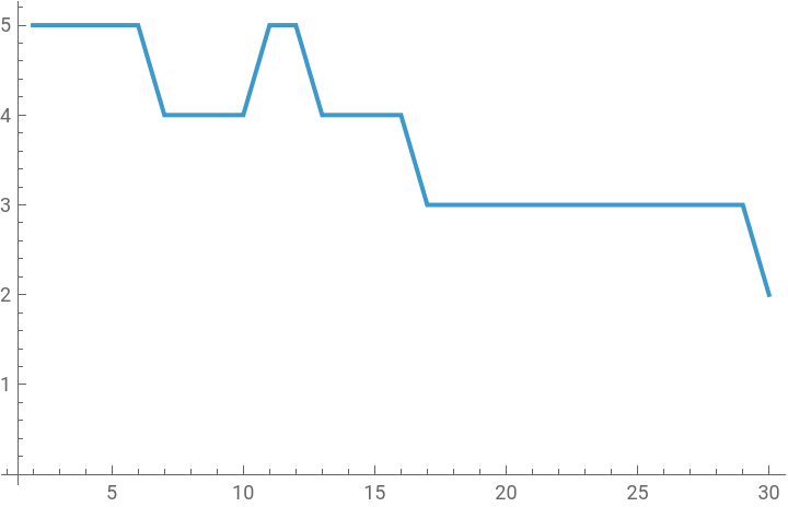
The most notable structural difference is that the modular graph spikes midway through, while no maximum restricted graph is able to do so. That being said, there are many other differences between the two types of graphs: modular graphs don’t fall to two iterations after reaching the halfway point and the starting equilibrium value varies.
When we consider only the primes, the result also deviates from its maximum restricted counterpart.
Out[]=
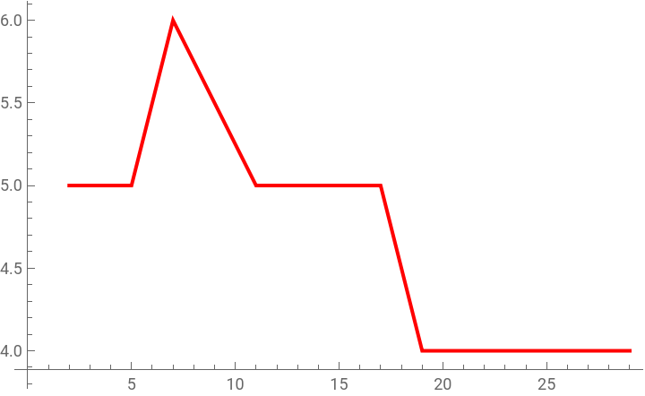
Again we see that using the modular restriction allows for an increase in the equilibrium value as the modular graphs are inherently more complicated.
Out[]=
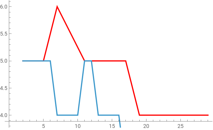
The effect of adding the non-prime generators in the case of a modular restriction is less predictable than the maximum restriction.
Increasing Restraints
Increasing Restraints
Instead of looking at the effect of adding generators, we can also look at the effect of increasing the max value. Intuitively, as the max value increases, so to does the required number of iterations for the multiplicad to reach equilibrium. Starting at 1, once the max number reaches the smallest generator squared it jumps to 2 iterations.
Out[]=
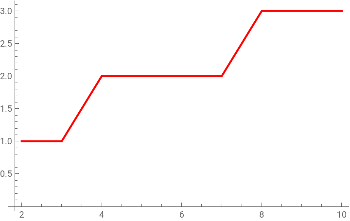
Similarly as with increasing the generators, if all the generators are co-primes, then the graph follows the behavior of the smallest prime. However, if the generators are not relatively prime, then adding more generators changes the graph behavior such that it takes the same or less iterations to reach the same max value.
Using a basis of Log(x), 1/Log(x),... we can create functions to model these graphs with non co-prime generators. With accurate enough models, it should be possible to calculate the difference in the rate of growth by taking the integral from 2 to infinity of the second derivative of the difference of the two functions. However, making accurate enough functions to do this requires more points than I was able to generate.
Complex Generators
Complex Generators
Spirals in complex plane
Spirals in complex plane
The idea of the multiplicad is based around using positive integers as generators. However, we can expand upon it by allowing for complex generators. This quickly complicates the graph.
For better visualization, we can plot the same relation onto the complex plane.
Shapely Values
Shapely Values
What they are
What they are
In cooperative game theory there is something called a Shapely value. The Shapely value is used to measure the impact that each individual has on the outcome of the game. This is done so by running trials of every subgroup of all the players and comparing the two subgroups which occur when 1 player is removed from a given subgroup
How they are applied
How they are applied
While there are no players involved in generating multiplicads, there are the generators. Thus, by treating each generator as a player, we are able to calculate the corresponding Shapley value of each generator. This allows us to quantitatively measure the impact of each generator the properties of the resulting multiplicad.
All the Shapley values for prime numbers are non-negative as it is impossible for a prime number to generate a number which has already been generated. Hence it can not lower the equilibrium value or any of the path lengths. Non-prime numbers, especially powers of primes, have a strong negative effect on all the measurements, except the percentage of numbers less than the maximum generated. This is because those numbers make short cuts where it would take other generators several iterations to produce the nodes they can produce in a single iteration. As they grow, the primes have less and less of an effect on the multiplicad because they cannot fit as many iterations into the same distance.
When a modular restriction is used the table for the same generators looks drastically different.
In modular restriction, the sign and magnitude of the Shapley values appear random. The generator 2, which consistently had one of the greatest impacts in the maximum restriction, has no effect on the equilibrium value or the longest shortest path length.
Concluding Remarks
Concluding Remarks
The multiplicad is a fascinating structure, with many properties related to whether or not the generators are relatively prime to each other as well as other properties which are entirely unrelated. All numbers grow the multiplicad in overall size. However, it is typically only the prime numbers that grow many of the properties of the maximum restricted multiplicads. The modular restricted multiplicads may be predictable, but I found no way to do so. There is still much to be found regarding all the methods of exploration used throughout this post.
Acknowledgments
Acknowledgments
My mentor for this project, Zsombor Méder, helped me significantly throughout the process of examining these properties. He was particularly helpful in writing code for several of the functions used throughout this document. Additionally, this project would not be made possible without the work of Stephen Wolfram and him suggesting this topic to me. Thank you to the both of them.
References
References
Wolfram, S. (2021, November 10). The concept of the Ruliad. Stephen Wolfram Writings. writings.stephenwolfram.com/2021/11/the-concept-of-the-ruliad.
Cite This Notebook
Cite This Notebook
Evaluating the Multiplicad
by John Cantwell
Wolfram Community, July 7, 2025
https://community.wolfram.com/groups/-/m/t/3497488
by John Cantwell
Wolfram Community, July 7, 2025
https://community.wolfram.com/groups/-/m/t/3497488