ABSTRACT (original article): We propose a novel family of entanglement measures for time-separated subsystems. Our definitions are applicable to any quantum system, continuous or discrete. To illustrate their utility, we derive upper and lower bounds on time-separated correlation functions, akin to the bound on spatially separated correlators in terms of the mutual information. In certain cases our bounds are tight. For relativistic quantum field theories our definition agrees with the analytic continuation from spacelike to timelike separated regions. We provide relevant measurement protocols and execute them on the IBM quantum device ibm_sherbrooke for a simple qubit system. Also we perform explicit computations for an Ising spin chain, free fermions, (1+1)-dimensional conformal field theories and holographic theories. Finally we explain how the proposed entanglement in time provides a microscopic definition for the recently introduced timelike pseudoentropy. CITATION (original article): Alexey Milekhin, Zofia Adamska, John Preskill (2025), arXiv:2502.12240. https://doi.org/10.48550/arXiv.2502.12240
This notebook reproduces Figures 3 and 4 from the paper above, as outlined in the Appendix F. The main idea is to use the definition of time-like density matrix T and adapt the Gaussian correlation matrix formalism of Peschel, https://arxiv.org/abs/cond-mat/0212631
For free fermions at zero temperature the correlation function (0,0)〉 is given by corr[t,x]
A related correlation function(0,0)〉 can be simply computed by multiplying by Exp[I Pi x]
〈(t,x)ψ
ψ
A related correlation function
〈ψ(t,x)
ψ
corr[t_,x_]:=-tHypergeometricPFQRegularized{1},,,-+2HypergeometricPFQRegularized{1},1-,1+,-;corrC[t_,x_]:=Exp[IPix]corr[t,x];
1
4
3-x
2
3+x
2
2
t
4
x
2
x
2
2
t
4
The correlation function (0,0)〉 can be computed from the first principles by using creating-annihilation operators. The resulting integral can be computed exactly yielding the expression above:
〈(t,x)ψ
ψ
IntegrateExp[It(-Cos[k])+Ikx],{k,-Pi/2,Pi/2}
1
2Pi
Out[]=
1
4
3-x
2
3+x
2
2
t
4
x
2
x
2
2
t
4
SpectrumTime[] is the main function here. It purpose is to form the correlation matrix CM (eq. (F3) in the paper ) of the following form = where i,j run through all possible fermionic operators in the intervals A and B. Specifically, CM has the following block-form:CM= where block GXX correspond to correlators within the intervals A,B and GTX and GXT correspond to cross-correlators.According to the original paper by Peschel (https://arxiv.org/abs/cond-mat/0212631), if CM has eigenvalues , then the reduced density matrix ρ has the following tensor product decomposition:ρ=
...Here we generalizing this to the time-like density matrix T
CM
i,j
ψ
i
ψ
j
GXX | -GXT |
GTX | GXX |
λ
a
λ 1 | 0 |
0 | 1- λ 1 |
λ 2 | 0 |
0 | 1- λ 2 |
SpectrumTime takes the following arguments:
L - the length of two intervals (they are assumed to be equal).
pos - is the relative shift between the two: one interval can be assumed to be [0,L] and the other one [pos,L+pos].
t - time-separation between them.
acc - accuracy of computing eigenvalues.
L - the length of two intervals (they are assumed to be equal).
pos - is the relative shift between the two: one interval can be assumed to be [0,L] and the other one [pos,L+pos].
t - time-separation between them.
acc - accuracy of computing eigenvalues.
For large intervals one needs more than machine precision. This problem is present in the standard entanglement entropy computations using correlation matrices
For optimization, we can use the fact that corr[0,x] has simple form. Also we used a “dynamical programming” trick by computing corr[t,x] for different x before populating the matrices GTX and GTX and GXX.
Sin[Pi/2(x)]
Pi(x)
SpectrumTime[L_,pos_,t_,acc_]:=Blockgxx=ParallelTableIfx0,,N,acc,{x,-L,L},gtx=ParallelTable[N[corr[t,x],acc],{x,-L-pos-1,L+pos+1}],twist=Table[Exp[IPix],{x,-L-pos-1,L+pos+1}],,gxt,GXX,GTX,GXT,CM,gxt=twistReverse[gtx];GXX=Table[gxx[[i-j+(L+1)]],{i,1,L},{j,1,L}];GTX=Table[gtx[[i-j+(L+pos+2)]],{i,1+pos,pos+L},{j,1,L}];GXT=Table[gxt[[i-j+(L+pos+2)]],{j,1,L},{i,1+pos,L+pos}];CM=ArrayFlatten[{{GXX,-GXT},{GTX,GXX}}];Eigenvalues[CM]
1
2
Sin[Pi/2(x)]
Pi(x)
These two auxiliary functions compute -Tr T log[T] and Tr given the eigenvalues of the correlation matrix
n
T
vNEntropy[gs_]:=-Total[gsLog[gs]+(1-gs)Log[1-gs]];Renyi[gs_,n_]:=Product[+,{i,1,Length[gs]}];
n
gs[[i]]
n
(1-gs[[i]])
Computing spectrum of CM for various time separations
In[]:=
ts=Subdivide[2,150,75];spc=Monitor[Table[SpectrumTime[50,70,t,20],{t,ts}],N[t]];
Export["/home/alex/spc_L50.dat",spc]
Out[]=
/home/alex/spc_L50.dat
Computing the entropies
r2s=Table[Renyi[gs,2],{gs,spc}];
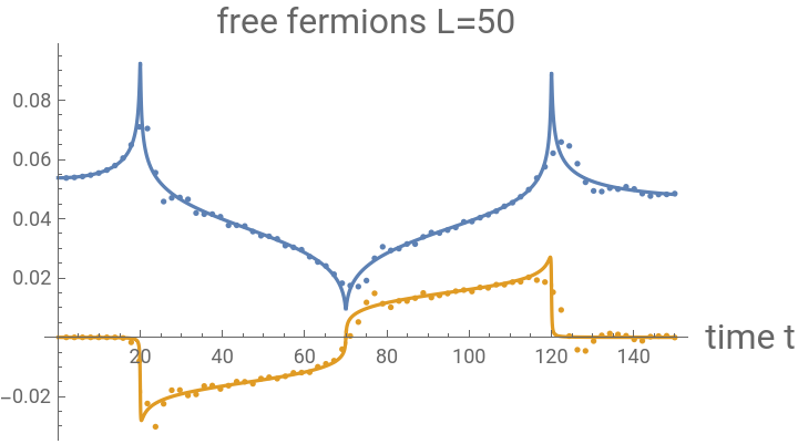
Using the notation above, the second moment Tr for free fermion conformal field theory (CFT) is given by eq. (38) in the paperTr =Note that CFT prediction does not give the precise numerical coefficient, which is related to the short-distance cutoff. However, this coefficient does not depend on L, pos or t, this is why we can perform a meaningful comparison between the lattice numerics and the CFT answer.
2
T
2
T
-1/8
(-L-pos-t)(L-pos-t)(-L-pos+t)(L-p+t)
2
(-pos-t)
2
(-pos+t)
Clear[tc];ϵ=0.1;tc=t-ϵI;(*standardinrelativisticquantumfieldtheories(RQFT)iϵprescription*)L=50;pos=70;fullplot=ShowPlot0.045Re,0.045Im,{t,0,150},PlotPoints10000,AxesLabel{Style["time t",16]},PlotLabelStyle["free fermions L=50",16],PlotLegendsPlaced[{"Re Tr()","Im Tr()"},Below],ListPlot[{Transpose[{ts,Re[r2s]}],Transpose[{ts,Im[r2s]}]}]
-1/8
(-L-pos-tc)(L-pos-tc)(-L-pos+tc)(L-pos+tc)
2
(-pos-tc)
2
(-pos+tc)
-1/8
(-L-pos-tc)(L-pos-tc)(-L-pos+tc)(L-pos+tc)
2
(-pos-tc)
2
(-pos+tc)
2
T
2
T
Out[]=


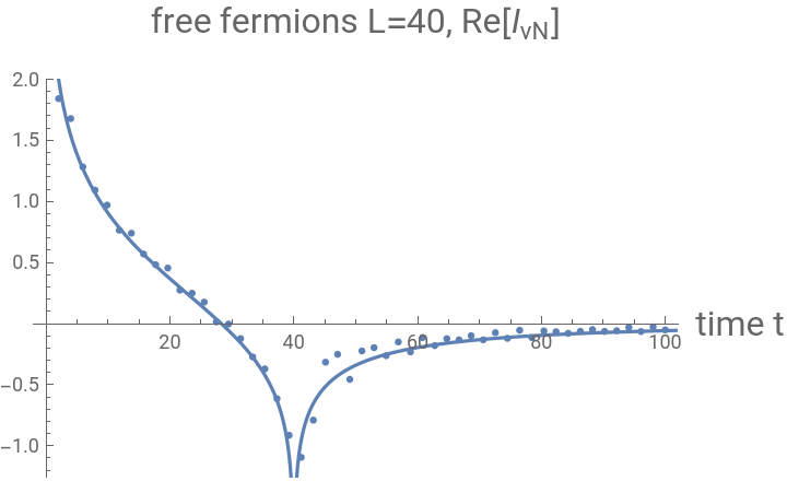
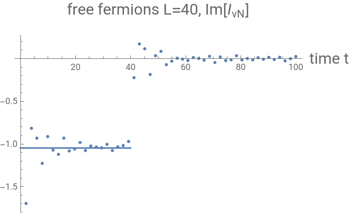
Similar computation but for two intervals of length 40 on top of each other. As mentioned in the main text, the correlation matrix eigenvalues are complex, so we are using the principle branch of the logarithm provides by Mathematica’s Log[] function. Constant shift -3.9 comes from von Neumann entanglement entropy of two intervals which can be computed in a similar way
ts2=Subdivide[2,100,50];spc2=Monitor[Table[SpectrumTime[40,0,t,20],{t,ts2}],N[t]];
vNs=Table[vNEntropy[gs],{gs,spc2}];
replot=ShowListPlot[{Transpose[{ts2,Re[vNs]-3.9}]},PlotRangeFull,PlotLabelStyle["free fermions L=40, Re[]",16],AxesLabel{Style["time t",16],""}],PlotReLog1-/.{Lc40},{t,1,150},PlotRangeFull
I
vN
1
3
2
Lc
2
t
Out[]=
implot=Show[ListPlot[{Transpose[{ts2,Im[vNs]}]},PlotLabelStyle["free fermions L=40, Im[]",16],AxesLabel{Style["time t",16],""}],Plot[-Pi/3,{t,0,40}]]
I
vN
Out[]=
CITE THIS NOTEBOOK
CITE THIS NOTEBOOK
Observable and computable entanglement in time
by Alexey Milekhin, Zofia Adamska & John Preskill
Wolfram Community, STAFF PICKS, April 25, 2025
https://community.wolfram.com/groups/-/m/t/3450948
by Alexey Milekhin, Zofia Adamska & John Preskill
Wolfram Community, STAFF PICKS, April 25, 2025
https://community.wolfram.com/groups/-/m/t/3450948