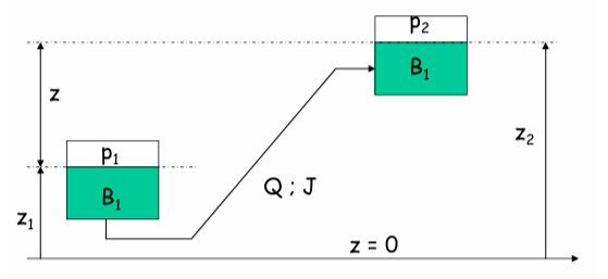
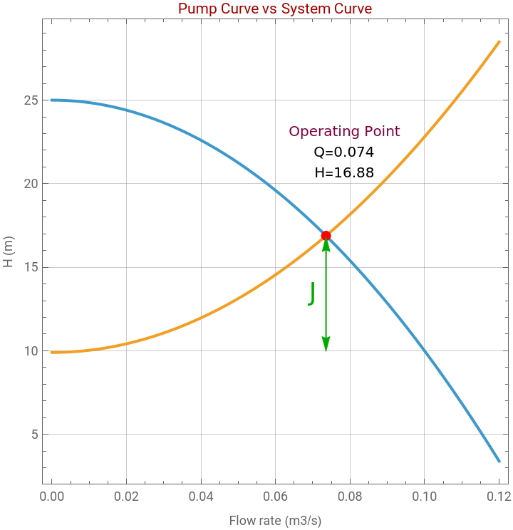
The operating point of a pumping system is determined by the intersection of the pump characteristic curve and the system resistance curve. The pump curve represents the relationship between pump head and flow rate, while the system curve represents the total head required by the piping network, including elevation difference, pressure difference, and friction losses.
Here, water is pumped from one point to another with an elevation increase of 15 m and a pressure drop between the inlet and outlet of 0.5 bar. The pump characteristic is modeled by a quadratic relation between head and flow rate, while friction losses in the pipeline are calculated using the Darcy–Weisbach formulation expressed in terms of flow rate.
The governing energy balance combines pump head, static head, pressure effects, and friction losses. Solving the pump equation together with the system equation gives the operating point of the system, corresponding to the actual flow rate and pump head during operation.
The graphical representation of both curves provides a clear visualization of system behavior. Their intersection defines the stable operating condition of the pump. For the selected parameters, the solution gives a flow rate of approximately 0.074 m³/s and a pump head of about 16.9 m, which is physically realistic and consistent with good engineering design practice.
Elevation
z1=0;z2=15;
Pressures at points 1 and 2
p1=1.510^5;p2=10^5;
Pump characteristics
a=25;b=1500;
Assume this friction factor
fA=0.05;
Pipe diameter
DA=0.2;
Pipe length
LA=100;
Water density
rho=1000;
In m/s2
g=9.81;
Governing equations
eq1=H+(z1-z2)+(p1-p2)/(rho*g)-0.81(fA*QA^2*LA)/(g*DA^5)==0;eq2=H==a-b*QA^2;
Solve using FindRoot
sol=FindRoot[{eq1,eq2},{{H,10},{QA,0.1}}];
Hsol=H/.sol;
QAsol=QA/.sol;
Print["Pump Head:"];
Print["H = ",NumberForm[Hsol,{6,4}]," m"];
Print["\nFlow rates:"];
Print["QA = ",NumberForm[QAsol,{6,4}]," m3/s"];
Pump Head:
H = 16.8838 m
Flow rates:
QA = 0.0736 m3/s
In[]:=
pump[Q_]:=a-bQ^2;
In[]:=
system[Q_]:=-(z1-z2)-(p1-p2)/(rho*g)+0.81(fA*Q^2*LA)/(g*DA^5);
Operating point
sol=FindRoot[pump[Q]-system[Q]==0,{Q,0.1}]
Out[]=
{Q0.0735581}
In[]:=
hG=-(z1-z2)-(p1-p2)/(rho*g)
Out[]=
9.90316
In[]:=
Qop=Q/.sol;Hop=pump[Qop];
Plot{pump[Q],system[Q]},{Q,0,0.12},(*Jrepresentsthefrictionlosses*)
Out[]=


CITE THIS NOTEBOOK
CITE THIS NOTEBOOK
Operating point determination using pump curve and system curve intersection
by Housam Binous
Wolfram Community, STAFF PICKS, April 26, 2026
https://community.wolfram.com/groups/-/m/t/3704299
by Housam Binous
Wolfram Community, STAFF PICKS, April 26, 2026
https://community.wolfram.com/groups/-/m/t/3704299