ORIGINAL ARTICLE: S. Hutzler, J. Ryan-Purcell, A. Mughal and D. Weaire (2023), A continuum description of the buckling of a line of spheres in a transverse harmonic confining potential. R. Soc. Open Sci. 10: 230293. http://doi.org/10.1098/rsos.230293
Article Abstract: A line of contacting hard spheres, placed in a transverse confining potential, buckles under compression, or when tilted away from the horizontal, once a critical tilt angle is exceeded. This interesting nonlinear problem is enriched by the combined application of both compression and tilt. In a continuous formulation the profile of transverse sphere displacement is well described by numerical solutions of a second order differential equation (provided that buckling is not of large amplitude). Here we provide a detailed discussion of these solutions, which are approximated by analytic expressions in terms of Jacobi, Whittaker, and Airy functions. The analysis in terms of Whittaker functions yields an exact result for the critical tilt for buckling without compression.
This notebook details the work done by the Foams and Complex Systems Group (led by Professor Stefan Hutzler) in Trinity College Dublin, in collaboration with Dr Adil Mughal of Aberystwyth University Wales, on this topic. In here, the differential equation of interest is defined and solved, and its solutions correspond to the buckling profiles found in these 1D chains.
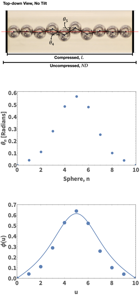
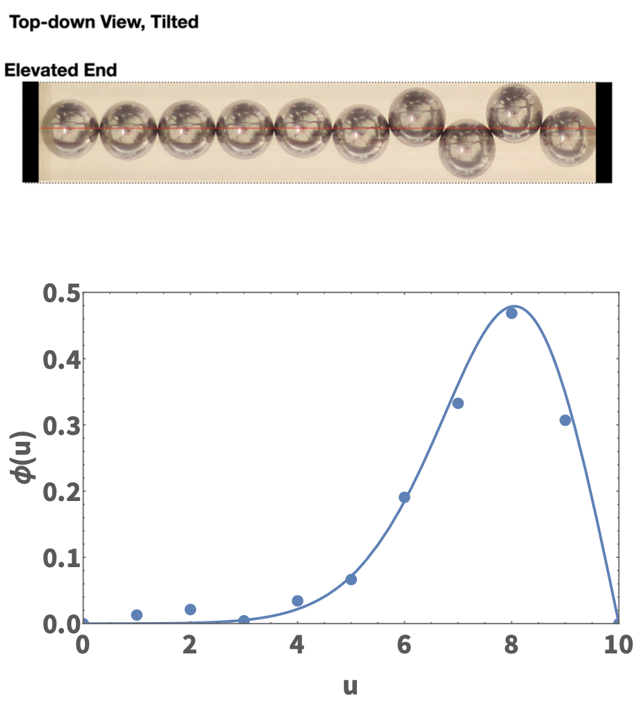
Examples of a simple experimental realisation of the system (ball bearings sitting on the curved surface of a cylinder), and the corresponding buckling profiles are shown below, for both the tilted and untilted cases:There are a number of quantities of interest in this system: - G : The compressive force exerted by the top wall on the system - Δ : The compression of the system, the difference between the natural and buckled chain lengths - τ : The longitudinal force applied to the system, or ‘tilt’. Here the solutions are presented for a system of N=10 spheres, however it can be in principle extended to systems of any length (see our previous paper: DOI 10.1103/PhysRevE.102.022905 ).
Full Differential Equation
Full Differential Equation
This is solved, for a given pair of , by Mathematica’s inbuilt NDSolve function. Helper functions are defined to implement a simple shooting method, designed to find the ‘symmetric’ solutions of interest that satisfy the boundary conditions.
{G,τ}
In[]:=
ClearAll[contSolNoShooting,endPointVal]contSolNoShooting[g0_?NumericQ,p1_?NumericQ,t_:0,n_:10]:=CheckNDSolveϕ''[u]-4ϕ[u]+,ϕ[0]0,ϕ'[0]p1,ϕ,{u,0,n},"Error"endPointVal[p_?NumericQ,g0_?NumericQ,t_?NumericQ]:=(ϕ[10]/.contSolNoShooting[g0,p,t,10])[[1]](*Weusethisfunctiontoimplementtheshootingmethodforfindingsolutionstothedifferentialequation*)Δ[sol_,n_?NumericQ]:=NIntegrate[1-Cos[ArcTan[ϕ[u]/.sol]],{u,0,n}](*Calculatingcompressionofasolutionasdiscussedinthepaper*)(*Foragiveng0,tpair,findthecorrectvalueoftheinitialslope,p.*)slopeFind[g0_,t_,guess_]:=FindRoot[endPointVal[p,g0,t],{p,guess},DampingFactor2,MaxIterations500]
ϕ[u]
(g0+t*u)
1+
2
ϕ[u]
In[]:=
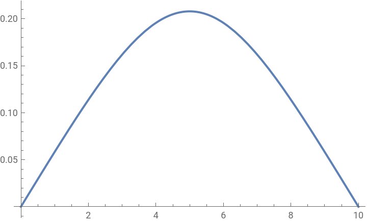
(*AsamplecalculationforN=10,t=0*)compressionG0[g0_?NumericQ,t_,s_]:=Module[{slopeOld,slopeNew,c},slopeOld=s;slopeNew=p/.slopeFind[g0,t,slopeOld];c=Δ[contSolNoShooting[g0,slopeNew,t],10];Return[{slopeNew,First[c]}]]compressionG0[0.252385,0,0.06]slope=%[[1]];Plot[Evaluate[ϕ[u]/.contSolNoShooting[0.252385,0.0586601916835453`,0,10]],{u,0,10}]
Out[]=
{0.0586602,0.100002}
Out[]=
Jacobi Solutions
Jacobi Solutions
Jacobi solutions are characterised by their values and produce solutions with 0 tilt. These can be determined by knowing the value of N and the target value of compression.
{,m}
2
κ
θcn[u_,k2s_,m_]:=ArcTan*JacobiCN(u),m;(*Note,thisisdefinedintermsofθratherthanϕ,hencetheArcTan*)(*AnexampleofaJacobisolution,withtheredsectionhighlightedshowingthepartofinterest*)m=0.6k=0.031Show[Plot[θcn[u-5,k,m],{u,0,10},PlotStyle{{Red,Dashing[0.02],Thickness[0.01]}}],Plot[θcn[u-5,k,m],{u,10,30},PlotStyle{{Thickness[0.01]}}],Plot[θcn[u-5,k,m],{u,-20,0},PlotStyle{{Thickness[0.01]}}],Plot[0,{x,-20,30},PlotStyleDashed],PlotRangeAutomatic,FrameLabel{"u","ϕ(u) (Jacobi profile)"}]
m*k2s
1+(2m-1)
k2s
4
k2s
2m-1
Airy Solutions
Airy Solutions
These are calculated using the rescaled variable x . After the rescaling, the solution can be written as a linear combination of Mathematica’s inbuilt AiryA and AiryB functions. The target compression can be matched with a scaling variable c
CITE THIS NOTEBOOK
CITE THIS NOTEBOOK
A continuum description of the buckling of a line of spheres in a transverse harmonic confining potential
by Stefan Hutzler, John Ryan-Purcell, Adil Mughal and Denis Weaire
Wolfram Community, STAFF PICKS, February 8, 2024
https://community.wolfram.com/groups/-/m/t/3118790
by Stefan Hutzler, John Ryan-Purcell, Adil Mughal and Denis Weaire
Wolfram Community, STAFF PICKS, February 8, 2024
https://community.wolfram.com/groups/-/m/t/3118790