Introduction
Introduction
The no-cloning theorem is one of the most fundamental results in quantum information theory: it states that it is impossible to create an identical copy of an arbitrary unknown quantum state. This limitation has profound implications for quantum communication, cryptography, and computation.
While perfect cloning is forbidden, approximate and probabilistic cloning schemes are possible. In this notebook, we explore three progressively refined approaches to quantum cloning. First, we examine the Wootters–Zurek cloning machine, which operates perfectly only for orthogonal states. Next, we analyze the universal quantum cloning machine, which produces approximate copies independently of the input state. Finally, we introduce a probabilistic protocol based on weak measurements that enhances fidelity at the cost of a reduced success probability.
Our goal is to illustrate how these different strategies arise from the constraints of quantum mechanics, and how additional information about the input state can be leveraged to improve cloning performance, using the Wolfram QuantumFramework:
The framework can be loaded with:
In[]:=
Needs["Wolfram`QuantumFramework`"]
Wootters–Zurek Quantum Copying Machine
Wootters–Zurek Quantum Copying Machine
To understand the limitations of quantum cloning, we begin with the original Wootters–Zurek protocol, which defines a cloning transformation that acts perfectly on a set of orthogonal basis states and, by linearity, extends to arbitrary input states. We therefore consider a general qubit expressed as a superposition of two orthogonal basis states and analyze how the cloning process behaves in this case. While the transformation acts perfectly on each basis element, its action on arbitrary superpositions reveals the fundamental limitations of the protocol.
Cloning Scheme
Cloning Scheme
We state the parameters constraints:
In[]:=
conds=(α|β)∈&&+==1;
2
α
2
β
The general state to be copied and its corresponding density matrix are given by:
In[]:=
ψ=QuantumState[{α,β}]
Out[]=
α|0〉+β|1〉
In[]:=
ρ=QuantumState[ψ["DensityMatrix"]]//FullSimplify[#,conds]&
Out[]=
2
α
2
β
Assuming perfect cloning, the corresponding two–dimensional ideal (id) state and its density matrix are given by:
In[]:=
ψid=QuantumTensorProduct[ψ,ψ]
Out[]=
2
α
2
β
In[]:=
ρid=QuantumState[ψid["DensityMatrix"]]//FullSimplify[#,conds]&
Out[]=
2
(-1)
2
β
3
α
3
α
2
α
2
β
3
α
2
α
2
β
2
α
2
β
3
β
3
α
2
α
2
β
|+|10〉〈10|+α|10〉〈11|+|11〉〈00|+α|11〉〈01|+α|11〉〈10|+|11〉〈11|
2
α
2
β
3
β
2
α
2
β
3
β
3
β
4
β
The cloning machine is defined by its action on the computational basis: and , where the indexes represent the input state (), the copy state (), and the machine state (). Applying this transformation to the general input state, we obtain:
|〉->|〉
0
s
0
s
0
c
0
m
|〉->|〉
1
s
1
s
1
c
1
m
s
c
m
In[]:=
ψscm=αQuantumState["000"]+βQuantumState["111"]
Out[]=
α|000〉+β|111〉
Cloning Performance
Cloning Performance
The resulting state is no longer a simple tensor product of identical copies; instead, it contains correlations between the system and the cloning machine, reflecting the imperfect nature of the cloning process. We now compute the corresponding density matrix:
In[]:=
ρscm=QuantumState[ψscm["DensityMatrix"]]//FullSimplify[#,conds]&
Out[]=
2
α
2
β
We trace out the machine to obtain the reduced density matrix of the original qubit and its clone:
In[]:=
ρsc=QuantumPartialTrace[ρscm,{3}]
Out[]=
2
α
2
β
We then take the partial trace to obtain the reduced density matrix of each qubit:
In[]:=
ρs=QuantumPartialTrace[QuantumState[ρsc],{2}]
Out[]=
2
α
2
β
In[]:=
ρc=QuantumPartialTrace[QuantumState[ρsc],{1}]
Out[]=
2
α
2
β
To quantify how close the cloned state is to the original, we introduce a performance measure based on the Hilbert–Schmidt distance between the cloned and original states. The definition of this function is given in Appendix A.
In[]:=
HilberSchmidtDistance[ρ,ρs]//FullSimplify[#,conds]&
Out[]=
2
Abs[α]Abs[β]We may also compute the distance between the ideal original–copy system and the actual original–copy system:
In[]:=
HilberSchmidtDistance[ρid,ρsc]//FullSimplify[#,conds]&
Out[]=
2
1-
Abs[β]2
β
In the Quantum Framework, the function already includes the option to compute the Hilbert–Schmidt distance directly:
QuantumDistance
In[]:=
QuantumDistance[ψ,ρs,"HilbertSchmidt"]//FullSimplify[#,conds]&
Out[]=
2-2
Abs[β]2
β
In[]:=
QuantumDistance[ψid,ρsc,"HilbertSchmidt"]//FullSimplify[#,conds]&
Out[]=
2
1-
Abs[β]2
β
The behavior of this measure is plotted as a function of the parameter :
β
In[]:=
Plot]Abs[β],{β,0,1},
2
Sqrt[1-2
β
Out[]=
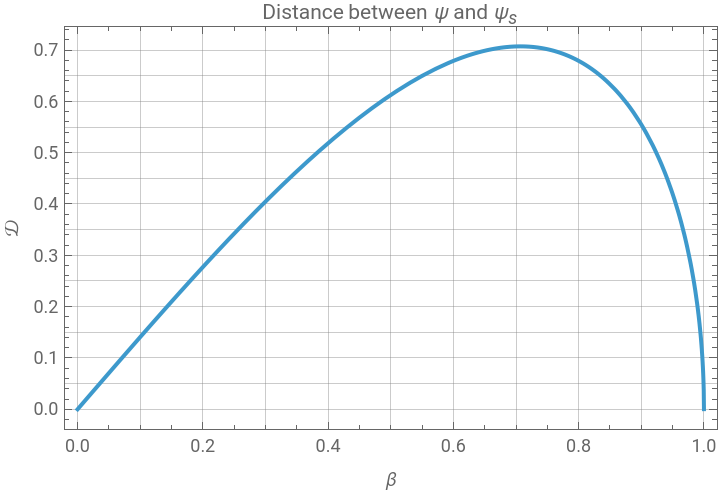
This plot shows that cloning becomes more difficult as the degree of quantum superposition increases. In particular, the error is maximal for balanced superpositions, where off–diagonal coherence is maximal.
Key Result
Key Result
The cloning is perfect for or , corresponding to the computational basis states. However, for intermediate superpositions, the distance between the cloned and original states is nonzero.
β=0
β=1
This result highlights a fundamental constraint of quantum mechanics: quantum information cannot be copied perfectly. Consequently, any practical cloning protocol must necessarily trade perfect copying for either reduced fidelity or probabilistic success.
Input State Independent Copying Machine
Input State Independent Copying Machine
As discussed in the previous section, the no-cloning theorem prevents the copying of an arbitrary quantum state with both unit probability and unit fidelity. However, it does not forbid the production of approximate copies with fidelity slightly less than one. In this section, following Bužek and Hillery [1], we aim to construct a machine that produces copies with the highest possible fidelity, independently of the input state.
Cloning Scheme
Cloning Scheme
The machine transform the basis states as follows:
|0〉
a
|Q〉
x
|0〉
a
|0〉
b
|〉
Q
0
x
|0〉
a
|1〉
b
|1〉
a
|0〉
b
|〉
Y
0
x
|1〉
a
|Q〉
x
|1〉
a
|1〉
b
|〉
Q
1
x
|0〉
a
|1〉
b
|1〉
a
|0〉
b
|〉
Y
1
x
where the machine states satisfy the following conditions:
2
x
Q
i
Q
i
x
2
x
Y
i
Y
i
x
x
Y
0
Y
1
x
,
x
Y
1
Y
0
x
x
Y
0
Y
0
x
=
x
Y
1
Y
1
x
x
Y
0
Q
1
x
=
x
Q
0
Y
1
x
=
x
Q
1
Y
0
x
=
x
Y
1
Q
0
x
First we introduce the following restrictions:
In[]:=
conds=(u|ξ|η)∈&&0<=u<=1&&0<=ξ<=1/2&&η^2<=4ξ(1-2ξ);
and then define the machine states as follows:
In[]:=
Withc=,q=1-2ξ,Q0=QuantumState,,0,0,
η
2
q
,0,0,0;Q1=QuantumState0,q
,0,0;Y0=QuantumState0,c
q
-+ξ
,0;Y1=QuantumState2
c
q
c
q
-+ξ
;2
c
q
Using the command defined in Appendix D, we verify that the machine states satisfy the conditions stated above:
DotProducts
In[]:=
DotProducts[{"Q0","Q1","Y0","Y1"},conds]
Out[]=
1-2ξ,0,0,,1-2ξ,,0,ξ,0,ξ
Q0
Q0
Q0
Q1
Q0
Y0
Q0
Y1
η
2
Q1
Q1
Q1
Y0
η
2
Q1
Y1
Y0
Y0
Y0
Y1
Y1
Y1
These conditions, together with the imposed restrictions, ensure the normalization and orthogonality properties required for the transformation to be physically valid.
Now, according to this cloning scheme, the state to be copied and its corresponding density matrix are given by:
In[]:=
ψ=QuantumState
u
,1-u
Out[]=
QuantumState


In[]:=
ρ=QuantumState[ψ["DensityMatrix"]]//FullSimplify[#,conds]&
Out[]=
QuantumState

Assuming perfect cloning, the corresponding two–dimensional ideal (id) state and its density matrix are given by:
In[]:=
ψid=QuantumTensorProduct[ψ,ψ];ρid=QuantumState[ψid["DensityMatrix"]]//FullSimplify[#,conds]&;
We define variables for each element of the two-dimensional qubit basis:
In[]:=
{ψ00,ψ01,ψ10,ψ11}=QuantumBasis[{2,2}]["BasisStates"];
The output states of the system, following the action of the machine on the computational basis, are given by:
In[]:=
ψ0=QuantumTensorProduct[ψ00,Q0]+QuantumTensorProduct[ψ01+ψ10,Y0]
Out[]=
1-2ξ
|0000〉+η
2
1-2ξ
ξ-
|0110〉+2
η
4(1-2ξ)
η
2
1-2ξ
ξ-
|1010〉2
η
4(1-2ξ)
In[]:=
ψ1=QuantumTensorProduct[ψ11,Q1]+QuantumTensorProduct[ψ01+ψ10,Y1]
The state corresponding to a general input take the form:
The corresponding density matrix is:
Cloning Performance
Cloning Performance
Distance Calculation
Distance Calculation
By tracing over the machine states, we obtain the density matrix of the original qubit and its copy:
We then trace over one of the remaining subsystems to obtain the reduced density matrix of one of the clones:
As in the previous section we compute the cloning performance using the Hilbert–Schmidt distance:
This expression shows how the distance depends on both the machine parameters and the input state, highlighting the need to impose additional constraints to achieve state–independent performance.
Imposing State Independence
Imposing State Independence
With these parameters at hand, we can verify that both distances are independent of the input state and take the following values:
Cloning Machine Implementation
Cloning Machine Implementation
We implement a function that takes a pure quantum state as input and returns both the original state and its corresponding clone after passing through the cloning machine.
Definitions
Definitions
Utility to display the results:
Function to generate the clones using the universal cloning machine:
Examples
Examples
To better understand the behavior of the function, the following examples illustrate how it performs across different parameter values.
As noted by Bužek and Hillery, the cloning machine applies to general input states, not only to the restricted case considered in the previous section. Here, we illustrate the results with two examples:
Key Result
Key Result
In summary, state–independent cloning provides a universal strategy in which all quantum states are treated equally. Although perfect cloning is not achievable, the protocol guarantees a constant fidelity across all inputs, reflecting a fundamental trade–off between universality and accuracy.
Optimizing Average Fidelity with State–Dependent Cloning
Optimizing Average Fidelity with State–Dependent Cloning
Cloning Scheme
Cloning Scheme
We analyze this possibility by retaining the same cloning machine and introducing a more general input state, while imposing the following restrictions:
The corresponding ideal copy is given by:
We then compute the output state and the corresponding density matrix resulting from the action of the cloning machine, with its parameters left unspecified:
By tracing over the machine degrees of freedom, we obtain the two-qubit state of the original–copy system. Further tracing over one of the clones yields the reduced state of a single clone.
Cloning Performance
Cloning Performance
Rather than seeking a state-independent fidelity, we instead consider whether a state-dependent cloning machine can outperform the universal machine on average. To this end, we first compute the average fidelity as:
We then maximize the fidelity with respect to the machine parameters, obtaining:
To visualize this result, the following plot displays the state-dependent average fidelities, with the maximum of each highlighted by a red dot:
Key Result
Key Result
Probabilistic Cloning with Weak Measurement
Probabilistic Cloning with Weak Measurement
In this section, we investigate a probabilistic quantum cloning protocol in which a weak measurement is performed prior to the cloning stage. This preprocessing step effectively modifies the input states, rendering them more amenable to cloning.
We consider two known nonorthogonal states, one of which is randomly selected for cloning, and show that tuning the measurement strength can significantly enhance the cloning fidelity, at the cost of a reduced success probability.
In contrast to universal cloning, this approach exploits partial prior information about the input states and reveals a clear trade–off between cloning fidelity and success probability.
Optimal Cloning for Two States
Optimal Cloning for Two States
Before introducing the weak measurement to enhance the fidelity, we first investigate the optimal cloning of two nonorthogonal states.
We start by specifying the assumptions:
Next, we define the two nonorthogonal states to be cloned:
with overlap is given by
The qubit corresponding to the clone is prepared in the state |0⟩, and we assume that, after the cloning transformation, the resulting two–qubit state is given by:
The unitarity of the transformation imposes the following constraints:
Taking the partial trace over the clone, we obtain the reduced density matrix of a single copy:
Weak Measurement
Weak Measurement
Consider the orthogonal projectors onto the ∣ + ⟩ and ∣ − ⟩ basis states:
which form a resolution of the identity:
These operators satisfy the completeness relation:
Cloning Scheme
Cloning Scheme
To enhance the cloning fidelity, we employ a scheme in which two qubits are used as inputs: the first is prepared in the state to be cloned, while the second is initialized as a blank copy in ∣0⟩. The first qubit undergoes a weak measurement and, conditional on obtaining outcome 1, both qubits are subsequently fed into the cloning machine. The entire process is represented by the following quantum circuit:
Using the measurement operators introduced above, we determine the success probability for each of the two nonorthogonal input states:
The associated post–measurement states are:
To quantify the degree of similarity between the two states, we evaluate their overlap:
The weak measurement effectively reduces the overlap between the states, thereby increasing their distinguishability and facilitating the cloning process.
with overlap:
Cloning Performance
Cloning Performance
Having determined the post–measurement state, we now apply the cloning transformation following the same procedure as before. The resulting output states for each of the two nonorthogonal states are given by:
The fidelity between the original state and one of the copies can be expressed as:
Substituting back gives the corresponding fidelity:
Setting the fidelity to one gives the relation (see Appendix A for derivation):
Key Result
Key Result
The behavior observed in the plot highlights a central feature of the protocol: higher cloning fidelity (close to its maximum) is achieved by increasing the distinguishability of the input states via weak measurement. However, this enhancement comes at the expense of a reduced success probability, revealing an intrinsic trade–off between fidelity and success.
Weak Measurements Do Not Improve Fidelity
Weak Measurements Do Not Improve Fidelity
Having shown how weak measurements can enhance cloning for two known nonorthogonal states, we now extend this approach to a broader family of input qubits. We investigate whether partial preprocessing combined with a more flexible cloning map can yield a higher average fidelity over this state space.
Cloning Scheme
Cloning Scheme
Again, we start by specifying the assumptions:
We prepare the qubit corresponding to the clone in the state |0⟩, and we assume that, after the cloning transformation, the resulting two–qubit state is given by:
The normalization and orthogonality conditions are readily satisfied. Substituting the parametrized expressions gives:
We now define the general input state to be cloned as follows:
A key part of the cloning protocol is the definition of the weak measurement. Here, we implement it using the following operators:
These operators define a valid quantum measurement:
With these measurement operators at hand, we can now compute the probability of obtaining outcome 1 after the weak measurement, as well as the corresponding normalized post-measurement state:
Cloning Performance
Cloning Performance
Applying the cloning transformation to the post-measurement state, we obtain the resulting two-qubit state, consisting of the modified original qubit and its clone:
Tracing over one of the qubits, we obtain the state of a single clone:
Using this state together with the original state we intended to clone, we evaluate the fidelity, which serves as a parameter–dependent measure of how well the cloning process performs:
Since this computation can be time–consuming, we also provide a precomputed version:
To optimize the cloning protocol, we maximize the fidelity averaged over the state to be cloned. Working with the squared single–state fidelity makes this average amenable to symbolic integration. The detailed calculation is presented in Appendix C; here we provide the precomputed expression.
Optimizing the average fidelity numerically over the physically allowed parameter domain leads to the following result:
Using these suggested values as a starting point, we then perform further numerical exploration of the mean fidelity. This analysis leads to the following set of parameters that maximize the mean fidelity:
Finally, for the optimal set of parameters we obtained, we compute both the average fidelity and the probability of success of the cloning process:
Cloning Machine Implementation
Cloning Machine Implementation
We implement a function that takes a pure quantum state as input and returns both the original state and its corresponding clone after passing through the probabilistic cloning machine.
Definitions
Definitions
Utility to display the results:
Function to simimulate the weak measurement:
Function to generate the clones using the probabilistic cloning machine:
Examples
Examples
Key Result
Key Result
Conclusion
Conclusion
Taken together, these results reveal a clear hierarchy in quantum cloning: the less prior information is available, the stronger the limitations on achievable fidelity. The Wootters–Zurek machine is exact only on a known orthogonal basis, the universal machine reaches 5/6 for arbitrary inputs, and the weak–measurement protocol explored here, even with its additional freedom, does not beat that universal value on average. In this sense, quantum cloning is not simply forbidden, but rather governed by precise and meaningful trade-offs between prior knowledge, fidelity, and success probability.
References
References
[1]
Bǔzek, V., & Hillery, M. (1996). Quantum copying: Beyond the no-cloning theorem. arXiv. https://arxiv.org/abs/quant-ph/9607018
[2]
Wang, M.-H., & Cai, Q.-Y. (2018). High fidelity quantum cloning of two known nonorthogonal quantum states via weak measurement. arXiv. https://arxiv.org/abs/1806.08112
Appendix A
Appendix A
In this appendix we give some definitions that are useful for symbolic computations.
For two quantum states with given density matrices, the Hilbert–Schmidt distance between them is computed as:
Similarly, for the special case of one pure quantum state and one mixed quantum state, the fidelity is given by:
If quantum states are assigned to a set of variables, all inner products between them can be computed as follows (where the input list contains the variable names):
Appendix B
Appendix B
Applying these transformation rules to the stored fidelity and simplifying, we obtain:
Finally, setting the term in parentheses to zero yields the relation:
Appendix C
Appendix C
In this appendix, we compute the average fidelity 〈F〉 of the squared single–state fidelity, which is used to optimize the probabilistic cloning protocol.
We perform the integration in two steps, first integrating in ϕ:
Evaluating the integral yields an analytical form of the average fidelity that depends only on the machine parameters and the weak–measurement strength:
We therefore define the fidelity as a piecewise function:
Appendix D
Appendix D
In this appendix, we provide the code to generate the quantum circuit for the probabilistic quantum cloning machine:
CITE THIS NOTEBOOK
CITE THIS NOTEBOOK
No-cloning theorem: 5/6 fidelity is Bloch-sphere average-optimal; weak measurement breaks it
by Maurice Engelhard
Wolfram Community, STAFF PICKS, May 8, 2026
https://community.wolfram.com/groups/-/m/t/3713257
by Maurice Engelhard
Wolfram Community, STAFF PICKS, May 8, 2026
https://community.wolfram.com/groups/-/m/t/3713257