Crane control represents a quintessential and multifaceted control problem, where the primary objective is to govern the motion of a load suspended by the crane. This task encompasses not only the precise positioning of the load but also the control of its swinging motion, which can become a notoriously complex challenge.
The intricacy of this problem arises from the need to simultaneously track the desired trajectory and minimize the pendulation of the load. Since the control inputs are typically applied only to the trolley, the system is under-actuated, meaning that the control of the load’s pendular motions must be carried out indirectly. This indirect control requires a sophisticated understanding of the dynamics involved and often necessitates the implementation of advanced control strategies.
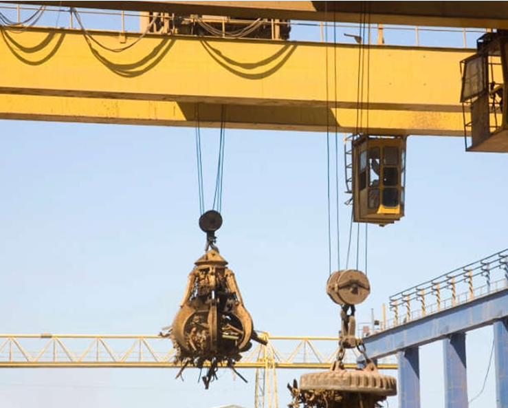
In this case study, a 3D model of a gantry crane is presented, comprising a trolley, hook, and load. The model is conceptualized as a double pendulum, where each pendulum exhibits two degrees of freedom. The cable connecting the gantry to the hook represents the length of the first pendulum, while the length from the hook to the load’s center of mass constitutes the second pendulum.
The control strategy employed in this example is a Linear Quadratic Gaussian (LQG) controller, designed to automate the control of the load swing during trolley movements. By combining the principles of Linear Quadratic Regulation (LQR) with a Kalman filter for state estimation, the LQG controller aims to achieve the desired positioning of the load with minimal swinging, even in the presence of disturbances or modeling uncertainties.
The following sections will delve into the mathematical formulation of the problem, the design of the LQG controller, and the simulation results that demonstrate the effectiveness of the proposed approach. Through this analysis, the reader will gain insights into the complexities and nuances of crane control, a problem that finds applications in various industrial settings and continues to be a stimulating area of research in the field of control systems engineering.
Mathematical Model
Mathematical Model
The system is a lumped model consisting of three main sections: the trolley, the hook and the load attached to hook. Using the Lagrangian formulation, each part’s kinetic and potential energies’ expressions are used to assemble the Lagrangian, from which the equations of motion are derived.
 |
|
The position and the velocity of the c.m. of the trolley:
In[]:=
0
x
0
y
0
0
0
Out[]=
{[t],[t],0}
′
x
0
′
y
0
The position and the velocity of the hook:
In[]:=
ℛ
1
θ
12
θ
11
1
0
ℛ
1
l
1
1
1
Out[]=
{Sin[[t]]+[t],Cos[[t]]Sin[[t]]+[t],Cos[[t]]Cos[[t]]}
θ
11
l
1
x
0
θ
11
θ
12
l
1
y
0
θ
11
θ
12
l
1
Out[]=
{[t]+Cos[[t]][t],[t]-Sin[[t]]Sin[[t]][t]+Cos[[t]]Cos[[t]][t],-Cos[[t]]Sin[[t]][t]-Cos[[t]]Sin[[t]][t]}
′
x
0
θ
11
l
1
′
θ
11
′
y
0
θ
11
θ
12
l
1
′
θ
11
θ
11
θ
12
l
1
′
θ
12
θ
12
θ
11
l
1
′
θ
11
θ
11
θ
12
l
1
′
θ
12
The position and the velocity of the c.m. of the load:
In[]:=
ℛ
2
θ
22
θ
21
2
1
ℛ
2
l
2
2
2
Out[]=
Sin[[t]]+Sin[[t]]+[t],Cos[[t]]Sin[[t]]+Cos[[t]]Sin[[t]]+[t],Cos[[t]]Cos[[t]]+Cos[[t]]Cos[[t]]
θ
11
l
1
1
2
θ
21
l
2
x
0
θ
11
θ
12
l
1
1
2
θ
21
θ
22
l
2
y
0
θ
11
θ
12
l
1
1
2
θ
21
θ
22
l
2
Out[]=
[t]+Cos[[t]][t]+Cos[[t]][t],[t]-Sin[[t]]Sin[[t]][t]+Cos[[t]]Cos[[t]][t]-Sin[[t]]Sin[[t]][t]+Cos[[t]]Cos[[t]][t],-Cos[[t]]Sin[[t]][t]-Cos[[t]]Sin[[t]][t]-Cos[[t]]Sin[[t]][t]-Cos[[t]]Sin[[t]][t]
′
x
0
θ
11
l
1
′
θ
11
1
2
θ
21
l
2
′
θ
21
′
y
0
θ
11
θ
12
l
1
′
θ
11
θ
11
θ
12
l
1
′
θ
12
1
2
θ
21
θ
22
l
2
′
θ
21
1
2
θ
21
θ
22
l
2
′
θ
22
θ
12
θ
11
l
1
′
θ
11
θ
11
θ
12
l
1
′
θ
12
1
2
θ
22
θ
21
l
2
′
θ
21
1
2
θ
21
θ
22
l
2
′
θ
22
The angular velocity of the load:
In[]:=
Ω
2
ℛ
2
ℛ
2
ω
2
Ω
2
Ω
2
Ω
2
Out[]=
{-Cos[[t]][t],[t],-Sin[[t]][t]}
θ
21
′
θ
22
′
θ
21
θ
21
′
θ
22
The kinetic energy of the system:
In[]:=
=.+.+.+.DiagonalMatrix[{,,}].
1
2
m
0
0
0
1
2
m
1
1
1
1
2
m
2
2
2
1
2
ω
2
ℐ
xx
ℐ
yy
ℐ
zz
ω
2
Out[]=
1
2
m
0
2
′
x
0
2
′
y
0
1
2
m
1
2
([t]+Cos[[t]][t])
′
x
0
θ
11
l
1
′
θ
11
2
([t]-Sin[[t]]Sin[[t]][t]+Cos[[t]]Cos[[t]][t])
′
y
0
θ
11
θ
12
l
1
′
θ
11
θ
11
θ
12
l
1
′
θ
12
2
(-Cos[[t]]Sin[[t]][t]-Cos[[t]]Sin[[t]][t])
θ
12
θ
11
l
1
′
θ
11
θ
11
θ
12
l
1
′
θ
12
1
2
ℐ
yy
2
′
θ
21
2
Cos[[t]]
θ
21
ℐ
xx
2
′
θ
22
2
Sin[[t]]
θ
21
ℐ
zz
2
′
θ
22
1
2
m
2
2
′
x
0
θ
11
l
1
′
θ
11
1
2
θ
21
l
2
′
θ
21
2
′
y
0
θ
11
θ
12
l
1
′
θ
11
θ
11
θ
12
l
1
′
θ
12
1
2
θ
21
θ
22
l
2
′
θ
21
1
2
θ
21
θ
22
l
2
′
θ
22
2
-Cos[[t]]Sin[[t]][t]-Cos[[t]]Sin[[t]][t]-Cos[[t]]Sin[[t]][t]-Cos[[t]]Sin[[t]][t]
θ
12
θ
11
l
1
′
θ
11
θ
11
θ
12
l
1
′
θ
12
1
2
θ
22
θ
21
l
2
′
θ
21
1
2
θ
21
θ
22
l
2
′
θ
22
Only the hook and load have potential energy terms, hence there are only two terms in the expression of the potential energy of the system:
In[]:=
=-g[[3]]-g[[3]]
m
1
1
m
2
2
Out[]=
-gCos[[t]]Cos[[t]]-gCos[[t]]Cos[[t]]+Cos[[t]]Cos[[t]]
θ
11
θ
12
l
1
m
1
θ
11
θ
12
l
1
1
2
θ
21
θ
22
l
2
m
2
The Lagrangian is assembled using the kinetic and potential energy terms:
In[]:=
ℒ=-//Simplify
Out[]=
1
2
θ
11
θ
12
l
1
m
1
θ
11
θ
12
l
1
θ
21
θ
22
l
2
m
2
m
0
2
′
x
0
2
′
y
0
m
1
2
′
x
0
2
′
y
0
θ
11
l
1
′
x
0
′
θ
11
l
1
′
y
0
θ
11
θ
12
′
θ
11
θ
11
θ
12
′
θ
12
2
l
1
2
′
θ
11
2
Cos[[t]]
θ
11
2
′
θ
12
ℐ
yy
2
′
θ
21
2
Cos[[t]]
θ
21
ℐ
xx
2
′
θ
22
2
Sin[[t]]
θ
21
ℐ
zz
2
′
θ
22
m
2
2
′
x
0
θ
11
l
1
′
θ
11
1
2
θ
21
l
2
′
θ
21
1
4
2
(2(Cos[[t]]Sin[[t]][t]+Cos[[t]]Sin[[t]][t])+(Cos[[t]]Sin[[t]][t]+Cos[[t]]Sin[[t]][t]))
l
1
θ
12
θ
11
′
θ
11
θ
11
θ
12
′
θ
12
l
2
θ
22
θ
21
′
θ
21
θ
21
θ
22
′
θ
22
2
′
y
0
1
2
l
1
θ
11
θ
12
′
θ
11
θ
11
θ
12
′
θ
12
l
2
θ
21
θ
22
′
θ
21
θ
21
θ
22
′
θ
22
The generalized coordinates of the system:
In[]:=
vars={[t],[t],[t],[t]};
θ
11
θ
12
θ
21
θ
22
Inputs of the system are taken as the position of the trolley , ), and the disturbance forces at the tip of the gantry (, ):
(
x
0
y
0
d
x
d
y
In[]:=
inps={[t],[t],[t],[t]}
x
0
y
0
d
x
d
y
Out[]=
{[t],[t],[t],[t]}
x
0
y
0
d
x
d
y
Generalized force comes from disturbance forces at the tip of the load and friction in the joints:
In[]:=
ℱ=[t]D[2[[1]],{vars}]+[t]D[2[[2]],{vars}]+{-'[t],-'[t],-'[t],-'[t]}
d
x
2
d
y
2
b
1
θ
11
b
1
θ
12
b
2
θ
21
b
2
θ
22
Out[]=
{2Cos[[t]][t]-2Sin[[t]]Sin[[t]][t]-[t],2Cos[[t]]Cos[[t]][t]-[t],Cos[[t]][t]-Sin[[t]]Sin[[t]][t]-[t],Cos[[t]]Cos[[t]][t]-[t]}
θ
11
l
1
d
x
θ
11
θ
12
l
1
d
y
b
1
′
θ
11
θ
11
θ
12
l
1
d
y
b
1
′
θ
12
θ
21
l
2
d
x
θ
21
θ
22
l
2
d
y
b
2
′
θ
21
θ
21
θ
22
l
2
d
y
b
2
′
θ
22
The equations of motion are derived by operating the Lagrangian with the Euler-Lagrange formula -=0:
d
dt
∂ℒ
∂q'
∂ℒ
∂q
In[]:=
eqns=Thread[Table[D[ℒ/.->0,q'[t]]-D[ℒ/.->0,q[t]],{q,vars/.var_[t]:>var}]==ℱ]//Simplify;Style[Grid[{%},Frame->All,Background{{None},{{LightGreen,LightBlue}}}],Small]
∂
t
m
0
m
0
Out[]=
Open-loop Simulation
Open-loop Simulation
A set of numerical values for the model parameters which are necessary to simulate the model:
Compute the state-space model of the system using the nonlinear equations of motion and the parameter values:
The output response to some initial conditions yields a highly oscillatory response as the pendulum and load swing about:
The response of the system to an disturbance force on the tip of the load is also oscillatory and unregulated:
Controller Design
Controller Design
The aim of the controller design is to obtain a controller than can regulate the load’s position. This is accomplished by dampening unforced response oscillations as well as the rejection of disturbances to the tip of the load.
A set of noise covariance matrices:
Using Bryson’s method, we can determine the values for state weights and control cost matrices. This involves setting the state weight as the square of the reciprocal of the maximum value of each state, while the control cost matrix is the square of the reciprocal of the maximum value for the controller inputs:
We can now compute the LQG controller:
Closed-loop Simulation
Closed-loop Simulation
With the controller as a data object, we can easily obtain the closed-loop system automatically as a property to simulate and assess the it’s ability to regulate the load’s position and rejection of disturbances. We can also inject noise into the system in order to assess the Kalman estimator’s filtering properties. Finally, we obtain the controller model, which will be used to assess the control effort of the closed-loop system.
The closed-loop system with controller in the feedback path:
To more accurately assess the closed-loop system’s performance, we introduce measurement and process noise. To do this, we generate two signals.
A noisy signal to simulate the process noise:
And another for the sensor noise:
The disturbance is rejected and the oscillations are damped:
Obtain the controller model:
CITE THIS NOTEBOOK
CITE THIS NOTEBOOK
3D modeling and control of a gantry crane
by Maher Kuzbari
Wolfram Community, STAFF PICKS, August 24, 2023
https://community.wolfram.com/groups/-/m/t/2997792
by Maher Kuzbari
Wolfram Community, STAFF PICKS, August 24, 2023
https://community.wolfram.com/groups/-/m/t/2997792