The project aims to analyze a simple 2D gas-like system in a container and look for the emergent properties of random behaviour in its constituent particles given specific initial conditions and cellular automaton evolution rules. These conditions can range from the introduction of a single or group of obstruction cells placed at specific coordinate location inside the container that interfere with the gas constituents to changing the initial number density, position or orientation of the gaseous constituents. This leaves a scope to evaluate and study a lot of inter-relationships between various measurable properties of the evolved system. The measurement of randomness and system’s ergodicity as a function of the perturbation strength and relative positioning, time/ensemble averages and autocorrelations of quantities like particle density distributions, cyclicity within the system as a function of time, are a few of those properties.
Table of Contents
Table of Contents
1
.Introduction
1
.1
.Outline of the Project
1
.2
.Introductory Remarks
2
.A system without obstruction cell
2
.1
.Block Cellular Automaton rules
2
.2
.Time snaps and space-time views
2
.3
.Analyzing the periodicity of the system
2
.4
.Relationship of periodicity with initial conditions
3
.An unobstructed system with rotated container
3
.1
.Block Cellular Automaton rules
3
.2
.Time snaps and space-time views
3
.3
.System’s Periodicity
3
.4
.Check for Ergodic Behaviour
4
.A system perturbed with obstruction cells
4
.1
.Block Cellular Automaton rules
4
.2
.Time snaps and space-time views
4
.3
.Periodicity
4
.4
.Ergodicity Analysis
◼
Concluding remarks and Future Work
◼
Keywords
◼
Acknowledgement
◼
References
◼
Appendix
1. Introduction
1. Introduction
1.1 Outline of the Project
1.1 Outline of the Project
As an outline, the basic goals of the project can be listed as:
◼
Study of 2nd law for the evolution of a simple gaseous model with or without perturbations.
◼
Quantifying randomness as a function of the initial conditions of the system.
◼
Measuring the cyclicity of the system’s evolution & then study the system’s ergodicity for a cycle time.
◼
Look for time averages of various quantities like density distributions, tail of the distribution etc.
◼
Establishing a relationship with the classical definition of entropy in the context of this computational model.
1.2 Introductory Remarks
1.2 Introductory Remarks
In the twentieth century, there emerged three great physical theories: general relativity, quantum mechanics and statistical mechanics, with the second law of thermodynamics being the defining phenomenon of statistical mechanics [1]. The aim of this project is to analyze the behaviour of a 2D gaseous system in context of the Second Law of thermodynamics. The essence of his theory lies in its ultimate foundation: the interplay between computational irreducibility and the computational boundedness of observers like us. In this project, we look upon such a gaseous system from the view-point of computational irreducibility.
Computationally irreducibility refers to the computations that cannot be speed up by means of any shortcut [2]. The principle of computational irreducibility says that the only way to determine the answer to a computationally irreducible question is to perform, or simulate, the computation. Some irreducible computations can be speed up by performing them on faster hardware, as the principle refers only to computation time. If the behavior of a system is obviously simple and is either repetitive or nested, then it is claimed to always be computationally reducible [1]. But it follows from the principle of computational equivalence that in practically all other cases it will be computationally irreducible. Here, “practically all” refers to cases that arise naturally or from a simple rule system as opposed to cases that are constructed artificially.
Now, if we go back to the origins of Second Law of thermodynamics, then we find that the earliest statements of the second law were things like: “Heat doesn’t flow from a colder body to a hotter one” or “You can’t systematically purely convert heat to mechanical work”. Later on there came the somewhat more abstract statement “Entropy tends to increase”. But in the end, all these statements boil down to the same idea: that somehow things always tend to get progressively “more random”. What may start in an orderly state will—according to the Second Law—inexorably “degrade” to a “randomized” state.
But how general is this phenomenon? Does it just apply to heat and temperature and molecules and things? Or is it something that applies across a whole range of kinds of systems across the universe?
The answer, according to Stephen Wolfram, is that underneath the Second Law there’s a very general phenomenon that’s extremely robust. And that has the potential to apply to pretty much any kind of system one can imagine. The key is to think in computational terms. And ultimately the source of the phenomenon is the interplay between the computational process associated with the actual evolution of the system and the computational processes that our perception of the output of that evolution brings to bear. We might have thought if a system had a simple underlying rule—like rule 30 [5]—then it’d always be straightforward to predict what the system will do. Of course, we could in principle always just run the rule and see what happens. But the question is whether we can expect to “jump ahead” and “find the outcome”, with much less computational effort than the actual evolution of the system involves. The answer seems to point in the direction of “computational irreducibility”, by virtue of which it should take an irreducible amount of computational effort to find out what the system does.
So how does the points talked about in the previous paragraph relate to the Second Law of thermodynamics? It’s what makes it possible for a system like rule 30 to operate according to a simple underlying rule, yet to intrinsically generate what seems like random behavior. If we could do all the necessary computationally irreducible work then we could in principle “see through” to the simple rules underneath. But the key point is that observers like us are computationally bounded in our capabilities. And this means that we’re not able to “see through the computational irreducibility”—with the result that the behavior we see “looks random to us”.
And in thermodynamics that “random-looking” behavior is what we associate with heat. And the Second Law assertion that energy associated with systematic mechanical work tends to “degrade into heat” then corresponds to the fact that when there’s computational irreducibility the behavior that’s generated is something we can’t readily “computationally see through”—so that it appears random to us.
So, based on the above discussions, we in the following sections study the evolution of a 2-dimensional gaseous system made up of hard spherical molecules. Depending on the initial conditions, the system may be divided into two categories namely unobstructed system and obstructed/perturbed system. The aim is to relate the evolutionary behaviour of such a system with the one predicted by the Second Law of thermodynamics. This may provide us with an insight into the basic principles/rules that universally governs an evolving system.
2. A system without obstruction cell:
2. A system without obstruction cell:
Initially, we focus ourselves to the case where the system evolves freely in a container without any perturbations or obstruction. The things to look for are the size of the gas container and size of gaseous system itself, both being measured in grid size and the initial position of gas molecules inside the container. These things form the basis for initial conditions of the system. Other than this, the rules that govern the evolution of system are also important and needs to be specified in advance. These rules are similar to the rules which are specified for a block cellular automaton.
2.1 Block Cellular Automaton rules
2.1 Block Cellular Automaton rules
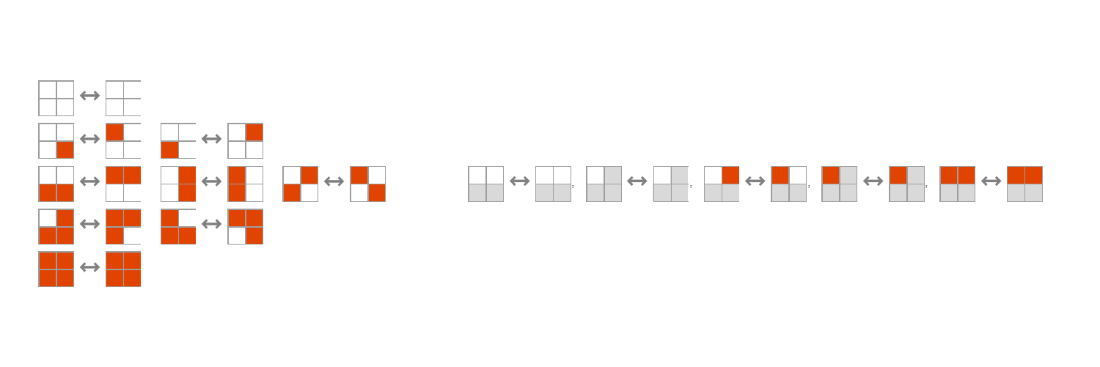
The graphics here depict the rules that a gas molecule follows through its evolution. These rules are specified for its movement through the container grid and also for the cases when it encounters either atleast one more gas molecule in its adjacent surrounding cells or the container wall in any of its adjacent surrounding cells.
Out[]=
2.2 Time snaps & space-time views
2.2 Time snaps & space-time views
In this section, we depict the evolution of our system by pictorial snap-shots of its evolution in a 2D grid-view. Also, to provide a continuum and fluid view of its evolution, we depict the dynamics of the system in 3D spacetime grid-view too. The space-time view is nothing but the stacked individual plots of 2D grid-view as time slices one over the other and then looked from an angled side-on view.
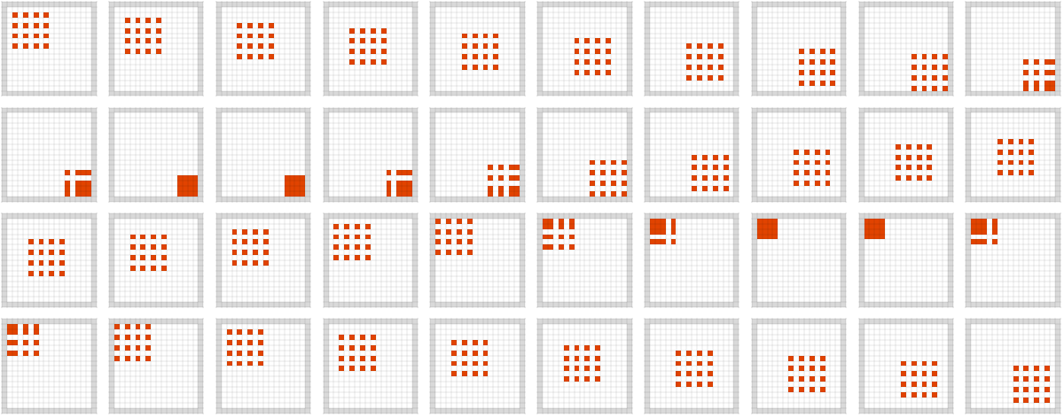
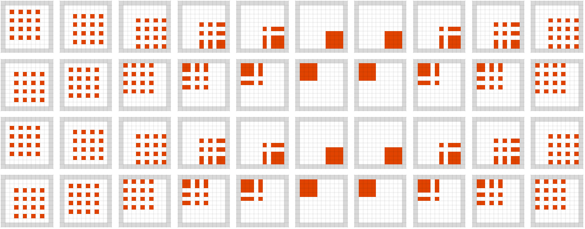
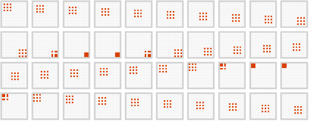
2D Grid-View for three systems with different initial states
2D Grid-View for three systems with different initial states
Here, we plot the evolution for three systems with a set of varying initial states so as to provide a graphical view of system’s behaviour under these conditions. In the first plot named “System 1”, we take the container of a 16x16 grid size with the gaseous system having a 4x4 molecular grid. Similarly, for the second plot named “System 2”, we reduce the container size to a 10x10 grid and for the third plot named “System 3”, we reduce the gaseous system to a 3x3 molecular grid.
Evolution with a specific Block cellular automaton rule and different initial conditions
Evolution with a specific Block cellular automaton rule and different initial conditions
The function defined below uses the Resource function BlockCellularAutomaton to generate a list depicting the evolution of a system. Here the function accepts 3 arguments as inputs. These arguments gg, cg and evo respectively decides the size of container and system and also the number of times the system is asked to evolve. The resource function used here has three options to be laid out for it. The rules for the system, the initial conditions and the number of system time evolutions, respectively.
In[]:=
grid[gg_,cg_,evo_]:=ResourceFunction["BlockCellularAutomaton"][],{2,2},{ArrayPad[Table[If[1<i<gg&&1<j<gg&&EvenQ[i]&&EvenQ[j],1,0],{i,cg},{j,cg}],1,2],0},evo;
This piece of code provides a graphical representation of the generated system information from the function grid above. The function depicts 0’s in list with White color (empty container cells), 1’s with red color (gas molecule filled cells).
In[]:=
GraphicsGridPartitionMapArrayPlotFirst[#],ImageSize->Full,ColorRules->0->White,1->["Reds",1],2->["Grays",1],Frame->None,Mesh->True,MeshStyle->GrayLevel[0,.05],ImageSize->Full&,grid[10,16,40],10
Out[]=
In[]:=
GraphicsGridPartitionMapArrayPlotFirst[#],ImageSize->Full,ColorRules->0->White,1->["Reds",1],2->["Grays",1],Frame->None,Mesh->True,MeshStyle->GrayLevel[0,.05],ImageSize->Full&,grid[10,10,40],10
Out[]=
In[]:=
GraphicsGridPartitionMapArrayPlotFirst[#],ImageSize->Full,ColorRules->0->White,1->["Reds",1],2->["Grays",1],Frame->None,Mesh->True,MeshStyle->GrayLevel[0,.05],ImageSize->Full&,grid[8,16,40],10
Out[]=
Visualizing the 3D space-time grid-view for one of the above systems
Visualizing the 3D space-time grid-view for one of the above systems
The code here plots a 3D representation of the above systems by exploiting the use of grid function defined above. The output of grid function is fed into an ArrayPlot3D function to visualize the data in 3D. The AddWalls resource function adds a wall to the grid to represent the container walls.
One may use the function grid to generate system with new initial conditions and then check their evolution visually in a 3D plot using the above code.
2.3 Analyzing the periodicity of the system
2.3 Analyzing the periodicity of the system
In this section, we quantify the periodicity for our system by finding the number of time evolutions that the system takes for completing one cycle of its behaviour. The system essentially repeats its behaviour after a cycle’s length.
The function below spits out the repeated part of the evolution for a BlockCellularAutomaton system. The function’s arguments gg and cg have the same meaning here as they have in a previous function named grid. The Table function at the end of the code creates the initial grid of the system and for changing the initial conditions, we need to modify the conditions written inside the Table function.
Repeating block for the system visualised in a 2D View
Repeating block for the system visualised in a 2D View
The code below make use of FindNestedTransientRepeat function from the Wolfram Function Repository to find the repeated part of system’s evolution. The output from this function is then fed into the ArrayPlot function to visualize the data. The colors of various types of cells are defined using the ColorRules option of ArrayPlot function.
Repeating block for the system in the 3D Space-time view along with its periodicity number
Repeating block for the system in the 3D Space-time view along with its periodicity number
The code below creates the 3D plot for the repeated part of our system’s evolution. By changing the initial conditions in the function named cycle, one may create new system and find their periodic part using this code. Other than the visual representation, the code also shows the numeric value for the time steps after which the system repeats itself.
2.4 Relationship between periodicity and initial condition
2.4 Relationship between periodicity and initial condition
As we see from the analysis done till now for a unobstructed gaseous system, the behaviour seems to be predictable and periodic. In this section, we visualize the dependence of system’s periodicity on some of its initial conditions. These initial conditions include the size of gas grid and container’s grid.
For a fixed size gas in a variable-grid container
For a fixed size gas in a variable-grid container
The code below creates a graphics using Manipulate to view the periodic block of system with a variable container size. The code uses the cycle function defined above to evolve the system.
For a variable-grid gas in a fixed size container
For a variable-grid gas in a fixed size container
The code below creates graphics using Manipulate to view the periodic block of system with a variable gas size. The code uses the cycle function defined above to evolve the system.
The code below makes use of the cycle function defined above to find the relationship of periodicity with an initial condition of the system by varying it step-wise while keeping the other initial condition constant and vice-versa.. The two plots are then plotted side-by-side using the GraphicsRow function.
From the plots above, we find that the periodicity of our unperturbed system depends on how far are the walls of container in which the gas is residing but not on the gas molecule number. This is due to the fact that even though by increasing the gas molecules we make the gas system bigger but a single molecule still has to make the same journey of covering the entire container length and getting back to its original position however big the total number of molecules there be, but by changing the size of container, we change the path that each gas molecule needs to cover for its entire journey and thus such a change directly alters the periodicity of the system.
Now, as per the analysis done in the entire previous section, we see that for the case of an unperturbed system with a head-on collision angle with the container’s wall, the evolution of the system necessarily remains periodic and reversible. The things here remain symmetrical enough that we don’t see any randomization—and in fact the only nontrivial thing that happens is a little Newton’s-cradling when the “caravan” of gas squares hits a wall. These type of well-behaved and rather simple systems are extremely rare to occur naturally in our universe at the sizes where statistical mechanics, relativity and quantum mechanics seem to work because even a slight deviation from a ideal behaviour (which is quiet likely in a system with many particles) can end the system up in a totally different evolutionary path. But nevertheless, this simplistic system seems to be a good starting point to study the group of such 2D gaseous systems.
So, now we plan to do better by making the system rules a bit complex. In the next section, we place the gas molecules in such a way that the collision between container walls and system is not head-on but at an angle. This results in a different overall dynamics of the system which we are gonna see below now.
3. An unobstructed system with rotated container
3. An unobstructed system with rotated container
In this section, we deal with the evolution of a system that has its container rotated by 45 degrees with respect to the setup discussed in the previous section. Such a rotation makes the system identical to the case of a system with “discrete velocity molecules” where the molecules not only have a velocity direction assigned to them from the start but are also spherical in shape instead of being perfect squares. The ideal scenario of a head-on collision taken in the previous case is no longer valid here, as the edges of gas molecules are not aligned with the walls of the container. This gives the system a chance to produce an intrinsic randomness in its behaviour given the fact that if two elastic spheres collide perfectly head-on, they’ll bounce back the way they came. But as soon as they’re even slightly off center they’ll bounce back at a different angle, and if they do this repeatedly even the tiniest initial off-centeredness will be arbitrarily amplified. A similar situation arises in this case too given the non-alignment of gas molecule edges with the container walls.
3.1 Block Cellular Automaton rules
3.1 Block Cellular Automaton rules
The graphics here depict the rules that a gas molecule follows through its evolution. The first column shows the rules already used in the previous section analysis. The second column shows a correspondence of these rules given a rotated container. The arrow-head signifies the direction of molecules’ movement. All these rules are specified for its movement through the container grid and also for the cases when it encounters atleast one more gas molecule in its adjacent surrounding cells.
3.2 Time-snaps and space-time views
3.2 Time-snaps and space-time views
Now, we focus our attention to visualize the evolution of our unobstructed system in a rotated container. Given the fact that a slight deviation from perfectly head-on collision can quickly escalate into a state with unpredictable behaviour, these visual representation will help us confirm the phenomenon. We need to keep in mind here that such a randomness is still intrinsic to the system and doesn’t involve any outside perturbation source.
Evolution of a gas system with rotated container using Block Cellular Automaton rules:
Evolution of a gas system with rotated container using Block Cellular Automaton rules:
This function below takes in three input parameters ggRot, cgRot and evoRot which decides the size of gas, size of container and system evolution steps, respectively. The function uses BlockCellularAutomaton to evolve the system according to the user-defined initial conditions. To create a rotated container, we make use of DiamondMatrix in-built function the input for which is taken from the cgRot parameter.
The code below makes use of rotgrid function to evolve our system with rotated container. The function’s values are fed to an ArrayPlot with specific color rules for each of the numbers 0, 1 & 2 present in it. The output generated from ArrayPlot is broken into sublists of 7 elements each, which is then represented visually using GraphicsGrid function.
From the plot above, we see that the system evolves to a non-ordered state starting with a highly ordered state. Now, as the system evolves into randomness, it would be interesting here to check whether our system has a periodicity in its behaviour and the dependence of that behaviour on system’s initial conditions. Also, we may check the possibility of ergodic nature in the system’s evolution. If our system happens to have a periodicity in its behaviour, then this points towards its pseudo-random nature instead of true randomness. Such periodicity would also hint towards the fact that if we start from any in-between random initial state of the system, the system after some time evolutions will go to a highly ordered state for a brief time.
Plot (space-time)
Plot (space-time)
Here, we plot the evolution of our system in a 3D space-time plot to better visualize its overall global behaviour.
The code below makes use of the rotgrid function to evolve the system, which is then represented visually using the ArrayPlot3D function with specific color rules defined for each of the array cell. AddWalls function adds walls to the 3D plot as a representation of the container’s walls in 3D. The time axis in these plots is from top to bottom for each plot.
Plot (side-on):
Plot (side-on):
Here, we visualize the evolution of our system in a side-on view of our 3D space-time plot. This side-on view incorporates the relevant dynamics that one needs to visualize while keeping the evaluation fast and computationally light.
The code below creates the mean of a single time slice(using in-built Mean function) over various columns into a single column. This necessary incorporates the effect of being looked from a side-on view. Other than that, we define two variables namely min and max to find the maximum and minimum value from the mean values of a particular time-slice, which is then used to create relative color rules for the visualization. This relative color grading is achieved by using the Blend function.
Plot (specific time-snaps)
Plot (specific time-snaps)
In order to get a feel of the system’s random behaviour, we plot here the evolution over longer time-scales of step size 50. From the images below, it can be clearly seen that system evolves towards a disordered state after around 200 time-steps. The plot here involves a 50x50 container grid with a 12x12 gas grid. Such a system is more complex in terms of the gas and container size compared with the previous analysis. For our analysis here, we define a new function that sets up the initial conditions for our rotated system and then evolve it over user given time steps. The result is fed to a ArrayPlot function to visualize the evolution with color rules defined for three different values (0,1 & 2) of our grid.
3.3 System’s Periodicity
3.3 System’s Periodicity
If we compare this system with the one analyzed in the previous section, we see a clear sign of randomness generation here. This randomness is purely intrinsic as the system doesn’t have an external source of perturbation introduced to it. So, once we have a disordered state, it would be interesting to check whether our system still remains periodic. Given the system shows periodic behaviour, we may check for the dependence of periodicity on the initial conditions of the system. Periodic nature of our system, if present would imply its pseudo-random nature instead of being truly random, as although the system might seem to diffuse to a disordered state over time, but after a period of evolution, the system is getting back to a ordered state, however big or small that period be.
High periodicity
High periodicity
For the case at hand, the system shows periodic behaviour over cycles of a fixed number of evolution steps. It is difficult to predict a general structure here, which allows us to foretell the periodicity of the system given an initial configuration. There are certain initial conditions for which the system seems to repeat itself after a relatively lower time evolutions. Below, we show two examples of such a case.
The code here takes in the full list containing information about the evolution of our system over “n” number of time steps and then find the repeating pattern in the list using in-built FindRepeat function. The numerical value of time step cycles over which system repeats itself is shown here. In the code after this, a visualization of system’s cycle is shown. The code marks the cycle by creating horizontal grey lines over those time steps from where the system starts to repeat itself. These points are identified by the locs variable in the code using which all such points in the dataset are replaced by their negative values. In order to produce a think grey line to clearly mark the cyclicity, the points just above and below the cycle points are also negated for their values. Then, inside the ArrayPlot function, a color rule is defined to mark all the negative elements of the list with in-built “Gray” color. Code makes use of rotgrid function defined earlier to evolve the system.
Low periodicity
Low periodicity
Here, we plot the behaviour of our system for a particular initial condition for which the system repeats itself after a comparatively larger number of time step evolutions. The overall structure of the code remains same here except the change in initial conditions defined for BlockCellularAutomaton function by tweaking the parameters of our self defined rotgrid function.
Based on the results in the sub-section above, one finds that the periodicity of systems which are still unperturbed from outside but have an intrinsic randomness to them, is affected not only by system size as in the case for totally unobstructed simple system discussed in first section, but also by the number of gas molecules. This behaviour of system adds one more layer to the overall complexity of the system as it changes the rather linear dependence of system’s periodicity on only the container’s size to a something more complex than a linear dependence. This analysis can be taken as a future extension of this work.
3.4 Check for Ergodic Behaviour
3.4 Check for Ergodic Behaviour
In the past one of the key ideas for the origin of Second Law-like behavior was ergodicity. And in the discrete-state systems we’re discussing here the definition of perfect ergodicity could be understood as: whatever state one starts from, one’s always guaranteed to eventually visit every possible other state [1]. In the context of this project, it could be understood as the tendency of gas molecules to visit every container cell if given a long time for the system to evolve.
But why is this relevant to the Second Law? In mathematics, ergodicity expresses the idea that a point of a moving system, either a dynamical system or a stochastic process, will eventually visit all parts of the space that the system moves in, in a uniform and random sense. This implies that the average behavior of the system can be deduced from the trajectory of a “typical” point. Equivalently, a sufficiently large collection of random samples from a process can represent the average statistical properties of the entire process. Ergodicity is a property of the system; it is a statement that the system cannot be reduced or factored into smaller components [4]. Also, we’ve said that the Second Law is about “degradation” from “special states” to “typical states”. And if one’s going to “do the ergodic thing” of visiting all possible states, then inevitably most of the states we’ll at least eventually pass through will be “typical”.
But why is this relevant to the Second Law? In mathematics, ergodicity expresses the idea that a point of a moving system, either a dynamical system or a stochastic process, will eventually visit all parts of the space that the system moves in, in a uniform and random sense. This implies that the average behavior of the system can be deduced from the trajectory of a “typical” point. Equivalently, a sufficiently large collection of random samples from a process can represent the average statistical properties of the entire process. Ergodicity is a property of the system; it is a statement that the system cannot be reduced or factored into smaller components [4]. Also, we’ve said that the Second Law is about “degradation” from “special states” to “typical states”. And if one’s going to “do the ergodic thing” of visiting all possible states, then inevitably most of the states we’ll at least eventually pass through will be “typical”.
Density Distribution Function
Density Distribution Function
In this subsection, we check the system for its ergodic nature by finding out the frequency of its visit to each and every accessible cell inside the container. For the same, we first plot out the matrix form of our system grid, where the numbers on the grid shows the no. of times a gas molecule has visited those cells. If the system is truly ergodic for a given initial conditions, then in principle, it should after a really long evolution have the frequency of visit for each of the system cell be equal to one another. Other than that, we also create a density distribution plot using ArrayPlot function to check the frequency of each system cell visit and also plot the Histogram for a better graphical representation of the same phenomenon. We use here rotgrid function defined earlier to evolve the system.
The plot here shows the density distribution of system’s cells after every 10 time steps of evolution starting from the initial configuration given using the function rotgrid. The plot can be tested for other initial configurations as well by tweaking the input parameters of the function.
Histogram
Histogram
The Histogram shown here related the frequency of gas molecules visiting a particular grid cell with the no. of cells that have that frequency. In a perfect ergodic system, such a Histogram must contain just a single peak at a value with no other bins in the Histogram representing that there is a equal probability of visiting the entire cells of the container while the system evolves. Although, even if the system might be truly ergodic, we will have to evolve it through a very long time to produce such a behaviour given the statistical nature of our system’s evolution.
The histogram and density distribution plot shows that the system prefers to stay in few specific cells of the container grid more than the other cells. Also, there seems to be a relation with these specific choices of cells with the initial placement of gas molecules within the container. Thus, choosing a different initial location of gas molecules might result in a different density distribution plot.
The analysis done in the previous subsection shows that the behaviour of our system is not truly ergodic as there is a higher probability of our system to visit some cells over the other. But such a claim is based on the evolution of system for a single initial state and more input would be needed to make a general statement about the system’s ergodic behaviour. Such an exercise can be taken as a part of future work of this project.
The analysis done in the previous subsection shows that the behaviour of our system is not truly ergodic as there is a higher probability of our system to visit some cells over the other. But such a claim is based on the evolution of system for a single initial state and more input would be needed to make a general statement about the system’s ergodic behaviour. Such an exercise can be taken as a part of future work of this project.
4. A system perturbed with obstruction cells
4. A system perturbed with obstruction cells
In this section, we notch up our system’s complexity by introducing external perturbation in the form of a rigid obstruction cell. This obstruction cell does not evolve with time and could be compared with the boundary of container in terms of its characteristics or its interaction with the gas molecules.
4.1 Block Cellular Automaton rules
4.1 Block Cellular Automaton rules
Here, we show the rules for the behaviour of system within the container for the case of external obstruction. On the left, the rules are for the case when a gas molecule is either freely evolving with no other gas molecule within its nearest neighbour distance or when the gas molecule is has a one or more than one gas molecule in its nearest surrounding cells. On the right, the rules are defined for the case when gas molecule has either a obstruction cell, one or more container walls in its nearest neighbour cells or a combination of obstruction and a second gas molecule in its surrounding nearest neighbour block.
4.2 Time-snaps and space-time views
4.2 Time-snaps and space-time views
Function to evolve the system
Function to evolve the system
The function here takes in four input parameters which are just defining the no. of gas molecules, size of container grid, placement of obstruction unit within the grid and no. of times system needs to be evolved, respectively.
Evolution in discrete time snap:
Evolution in discrete time snap:
The code below shows the evolution of system with an external rigid perturbation placed inside the container at a fixed position. From the output, we may see that the system quickly evolves from a highly ordered to a disordered state. This system may thus has been further analyzed for its periodicity and ergodicity. We also check the effect of introducing more than one obstruction inside the container grid on the emergent properties of system.
Evolution in 3D space-time grid (Time axis is top to bottom):
Evolution in 3D space-time grid (Time axis is top to bottom):
The function Row here presents the seven figures in a row without putting them within a list format, making the things presentable. AddWalls function adds a wall to the container at locations specified by the arguments inside it. ArrayPlot3D makes a array-plot in 3D for the list extracted through Resource function BlockCellularAutomaton. The BlockCellularAutomaton has three parameters as input first the rules for computation, second the initial conditions, where we are explicitly putting a obstruction at {9,9} and third the number of times the rule needs to be iterated. The Partition function has been used to break a single array of 700 elements to 7 arrays of 100 elements for better data visualization. The First function is applied to the level-2 inner layer of list produced through Partition to remove the extra 0, 1 coming with the lists. Also, the boundary wall for each grid has been removed by the Take function logic of selecting only from second to second last element in row and as well as in column.
Evolution in space-time grid with side-on view (Time axis is top to bottom)
Evolution in space-time grid with side-on view (Time axis is top to bottom)
The code here displays a row of 800 time-snap evolutions divided into 8 blocks of 100 steps each in continuation from top to bottom & left to right, in discrete mode of a perturbed cellular automaton with specific rules and initial conditions. Each graphic is spaced equally with 30 spacing using GraphicRow. The Module function is used to create the data-list of cellular automaton which is then fed to ArrayPlot to visualize it. In the cellular automaton, for every list element, we insert a obstruction cell at coordinate {9,9}. Then extract only the region of space within the boundary and exclude the boundary. This is done using the Take function with options as (2;;-2,2;;-2). Also, we then replace the {9,9} place with a 0. I don’t know why we did this. After that, we manipulate the data to find the mean of data along line of sight for every point on the plane so that we can compare the number of gas molecules across a line of sight for each column on the 2D list. This provides the correct picture of 3D space-time diagram projected on to 2D line of sight plane. We then get a 2D list to plot. This 2D list along with Min of data and Max of data is taken to the plotting function, where data is fed to ArrayPlot in 8 lists of 100 space-time points each by using Partition function. For every row data, the 9th point is the obstruction cell row, so if the value remains equals to zero(i.e. no gas molecule came along the line of sight of 9th row for that time-snap), then replace that value with the value of variable “w”, that is with grey color. If the value is not equal to zero, then replace it with the negative of whatever value is present. Then finally, we have the ColorRules function that is used to define the color of each pixel in the ArrayPlot. The value of a general pixel is defined by a function x which is defined as: If the value at a pixel is positive then Just blend two shades of red in a proportion defined by how much is the relative value of that pixel compared to other pixel values (given by blending amount: Abs[x]-min/max-min) in the Blend function. If the value is negative then, this value is fed into a pure function for further blending with Grey color. This is done to keep the greyness of obstruction cell intact to depict that it always is going through 9th row.
The use of Construct function with a If, Identity and pure function inside it, enables such implementation of color blending depending on pixel value.
The use of Construct function with a If, Identity and pure function inside it, enables such implementation of color blending depending on pixel value.
Evolving a system with multiple obstruction cells
Evolving a system with multiple obstruction cells
In this piece of code, we plot the time-snap view for a system with multiple rigid obstruction cells within the container grid. For a direct comparison to the previous case of single obstruction, we keep the other initial conditions of the system same. The Table function added at the end of our code inserts multiple obstruction cells in the code. Other than that, rest of the code remains same, if compared with the previous case of single obstruction cell.
From the above plot, it can be seen that with the introduction of more obstruction cells in the system, the overall behaviour of system becomes more random and less predictable. To quantify this, in the subsequent subsection, we compare the ergodicity of the system for the case of single and multiple obstruction cells while keeping other initial conditions same for both the cases.
4.3 Periodicity
4.3 Periodicity
The Histogram plotted here shows the behaviour of system’s periodicity with the changing initial conditions for the case of a 1D system defined for a size 17 gas molecules in a 30 celled container row. A lot of initial conditions can be formed by the combination of various available system configurations. We here use the already available dataset on wolfram repository containing a list of 2D lists with set of initial conditions for the system along with the periodicity number for that particular initial condition as the second element of each list. One may uniconize the dataSamples to view them. There are around 10000 different initial conditions along with their periodicity retrieved from the repository for a particular rule defined in the opening lines of this paragraph. All of them are fed into the variable “dataSamples” and then a histogram is plotted for the frequency of periodicity values. The histogram shows a clear tailed behaviour in its distribution which suggests that for a given rule and system size, there will always be few initial conditions with very high randomness and the system will repeat itself after a very long cycle. Given the time requirement for creating the data sets for this exercise in the case of a 2D system, the analysis has been left as an extension to this work. Appendix [1], contains the steps for creating those datasets and few of them have been created there. Although due to the lack of sufficient data, the histogram doesn’t resemble a tailed distribution and more datasets are required.
In Appendix [2], we present our analysis to find the numeric value of power-law for our distribution. As the analysis is still not thoroughly done and more concrete results can be found in future, so we found it best to keep it as an extra analysis section in Appendix of our project.
4.4 Ergodicity Analysis
4.4 Ergodicity Analysis
In this sub-section, we compare the ergodic behaviour of our system for the case of single and multiple obstruction cells. Thus, for this analysis, we plot the density distribution curves and the histograms for the two cases.
Density Distribution Function
Density Distribution Function
The code here creates a manipulative plot for the density distribution of gas molecules over the entire accessible container grid for both the cases to analyze. We evolve the system for a rather small time scale of 5000 steps so as to not make the code computationally heavy and also extract the difference in the behaviour of two systems. After starting with a similar set of initial conditions, we clearly can see that the two systems quickly evolve to different states in terms of their density distribution characteristics. The system with single obstruction has clearly a favourable path for the system’s evolution which is marked by its visit to few system cells more often than the others. Also, we can see here that there are few cells which are never visited by the system in this configuration. On the other hand, for the second system, we see that the states evolve in such a way that a more uniform probability is seen for the density distribution of gas molecules over the temporal evolution of the system. Although, a histogram based analysis will provide a better insight of the likelihood of gas molecules to visit the container grid with uniform probability.
Histogram
Histogram
A histogram comparing the 2 cases is plotted here. We see that for the single obstruction cell case, there is a moderate preference of gas molecules to visit most of the cells, a high preference to visit specific cells and almost zero preference to visit the remaining few cells. This type of behaviour signifies that the system overall has a preferred behaviour in its evolution. On the other hand, we see that by increasing the number of obstruction cells, we decrease this preferred behaviour of our system. This can be seen from the second plot, where most of the system cells are visited with equal likelihood. This behaviour can be understood from the shifting of sky scrapper in the plot from middle to right. This shift signifies that as the amount of obstruction in our system is increased, the system is equally likely to reach all the states and a clear preference to few states (as pointed in the first plot) decreases. This indirectly ensures a more random and ergodic nature of the system with the increase in obstruction.
Concluding remarks & Future Work
Concluding remarks & Future Work
Goal:
Goal:
The project aimed to track and analyze the evolution of a 2D gas with hard sphere molecules inside a container. As per the rules of Second Law of thermodynamics, such a system is doomed to evolve into a random, disordered state given some perturbation to the system. The goal was to study the effect of perturbations on the order of randomness in such a system. There are various other measurable quantities that emerge as individual defining characters of this system, such as system’s periodicity, ergodicity, density distributions and emergence of a tailed behaviour in its period frequencies. We incorporated in our analysis, a systematic study of these characteristics for various system configurations and different sets of initial conditions. Our goal also include a comment on the relationship of Second Law of thermodynamics with our system’s emergent behaviour and properties.
Main Results:
Main Results:
Within the three weeks of summer school, we established few critical connections regarding the periodicity of an unperturbed system with its initial conditions. We found out that the periodicity of such a system has a linear relationship with the size of container but is independent of the gas molecule number in the case of a truly simple system discussed in section 2 but for an unperturbed system with rotated containers we see that the periodicity of the system depends also on the gas molecule number and the overall effect of altering both the gas size and container size makes the relationship far from linear. We also found that in order to generate randomness in the system, it is not always essential to generate external perturbations. Given a gas in a rotated container (as discussed in section 3), i.e. a container with non-aligned container walls to the gas molecule edges or equivalently, a gas with molecules that are allowed to have non head-on collisions, we saw emergence of intrinsic random behaviour devoid of any external perturbation. For the case of externally perturbed gas system discussed in section 4, we observed that for most of the allowed initial set-ups, the system showed a periodic behaviour, sometimes being highly periodic and for other configurations, having a long periods. This periodicity frequency in the form of a histogram was also studied for its tailed behaviour and power-law analysis. we also tried establishing a relationship between system’s periodicity and amount of obstruction to the system by plotting the periodicity with the number of obstruction cells in the system, keeping the other initial conditions fixed. Finally, we also analyzed the ergodic nature of our system by plotting its density distribution plot for both the externally and internally perturbed case.
Future Work:
Future Work:
Given the relevance of Second Law on statistical evolution of systems, this project has a plethora of analysis that can be taken as an extension to the work. The studied systems can be made more complex and real-like by adding the effects of heat dissipation or other dissipative forces. Also, the system could be studied for auto-correlations within the evolution of gas molecules. The emergence of Second Law type behaviour in the context of work done by the system can be studied in great detail. Other than these extensions, such an analysis can also be done for a gaseous system in 3D or fractional dimensional space-time, to relate the emergent system behaviours more fundamentally with the thermodynamical concepts like entropy and arrow of time. As an immediate extension after the summer school, I would continue analyzing the power law distributions of the system for a combination of container and gas sizes. There also have been small comments made within the text at few places about the possibility of extension for that particular piece of work.
Keywords
Keywords
◼
Second Law of thermodynamics
◼
Block Cellular Automaton
◼
Randomness
◼
Periodicity
◼
Ergodicity
Acknowledgment
Acknowledgment
I am really grateful to Stephen Wolfram for giving me an opportunity to be a part of this summer school from Wolfram, also I thank him for selecting a really interesting project for me. I would like to thank my mentor Jon for his guidance and immense support throughout this project. He reviewed my work during all the crucial stages in these past three weeks. His humble and cheerful conduct motivated me a lot. Also, I would like to acknowledge my co-mentor Adiba for her valuable contributions to my project. Her knowledge and passion towards the work kept me motivated throughout. A big thanks to all the TAs who helped me with code related issues. I would also like to thanks Xerxes Arsiwalla for his timely checks on the progress of my project and his constant support. At the last, I would like to thank the organisers and all the other support staff for their assistance and management throughout the School.
References
References
Appendix
Appendix
1. To find a tailed distribution in the periodicity for the case of perturbed 2D gas system
1. To find a tailed distribution in the periodicity for the case of perturbed 2D gas system
Checking the matrix layout:
Checking the matrix layout:
Here, we show graphically the various initial system configurations subjected to different initial conditions. This gives the user a feel of what different initial conditions means in terms of gas molecule content, their relative positioning within the system and system size. The 2’s and 0’s here represent the container grid, with 2 being the walls of container(non-accessible by gas molecules) and 0’s being the empty container grids accessible by system through its evolution. 1’s here refer to the gas molecules.
Obtaining the data:
Obtaining the data:
Importing the data from cloud (Preferable):
Importing the data from cloud (Preferable):
2. Analysis for finding the power-law of the tailed distribution
2. Analysis for finding the power-law of the tailed distribution
In here, we plot the histograms for probabilities of periodicities without taking the “Log”. The aim is to find the fitting function for the histogram distribution. After having the fit function, one can use it in principle to find the power law for the data.
CITE THIS NOTEBOOK
CITE THIS NOTEBOOK
Study of Statistical evolution of a gaseous system as a consequence of iterative simple rule
by Utkarsh Patel
Wolfram Community, STAFF PICKS, July 12, 2023
https://community.wolfram.com/groups/-/m/t/2959142
by Utkarsh Patel
Wolfram Community, STAFF PICKS, July 12, 2023
https://community.wolfram.com/groups/-/m/t/2959142