Transient Rise of Mercury in a Barometer under Atmospheric Pressure
Authors: Housam Binous and Ahmed Bellagi
Transient Rise of Mercury in a Barometer under Atmospheric Pressure
Authors: Housam Binous and Ahmed Bellagi
Authors: Housam Binous and Ahmed Bellagi
We simulates the time-dependent rise of mercury in a vertical barometer tube under atmospheric pressure. To do so, we account for: Nonlinear inertia of the mercury column (𝑚(𝑡)=𝜌𝐴ℎ(𝑡)), Gravity as the restoring force, Viscous damping generalized for all flow regimes using a Reynolds-number-dependent friction factor (a smooth tube is assumed) as well as height-dependent damping, where friction grows as the mercury column rises.
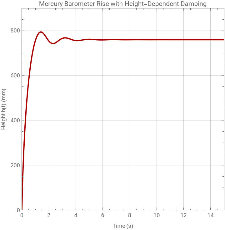
Starting from a small initial height, the mercury column accelerates due to atmospheric pressure, gradually slows due to viscous friction, and eventually reaches the equilibrium height (ℎ(∞)=𝑃atm/(𝜌𝑔)≈0.76 m).
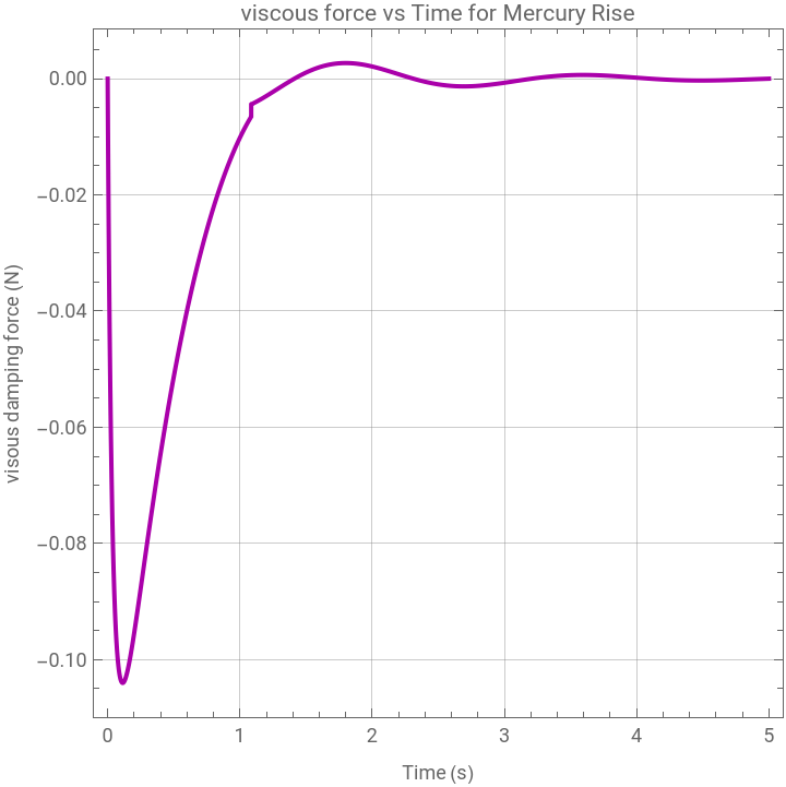
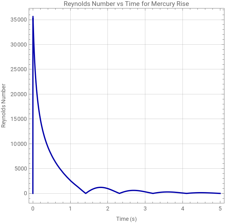
The model can also compute the Reynolds number of the rising column over time, illustrating the transitions from laminar to turbulent flow and the associated damping effects. Finally, we provide a plot of the viscous damping force (or the resistance due to the liquid’s viscosity as it moves along the tube walls).
This model constitutes a physically realistic transient simulation of the barometer response, including possible oscillations for low damping or smooth rise in highly damped tubes (narrow tubes).
In[]:=
Reynolds[t_]:=2RrhoAbs[h'[t]]/mu
In[]:=
Ffric[t_]:=Piecewise[{{8*mu*h[t]/R^2*A*h'[t],Reynolds[t]<2000},{0.3164*Reynolds[t]^(-0.25)*rho*A*h[t]/(4*R)*h'[t]^2,Reynolds[t]>=2000}}]
In[]:=
(*governingequation---Newton'ssecondlawofmotion---height-dependentdamping*)eqn=D[Arhoh[t]h'[t],t]+Ffric[t]+gh[t]Arho==PatmA
Out[]=
Agrhoh[t]+
+Arho[t]+Arhoh[t][t]APatm
|
2
′
h
′′
h
In[]:=
(*fuidproperties*)rho=13600;(*Mercurydensity,kg/m^3*)mu=1.526*10^-3;(*Mercuryviscosityat20°CinPa*s)
In[]:=
Patm=101325;(*Atmosphericpressure,Pa*)
In[]:=
g=9.81;(*Gravity,m/s^2*)
In[]:=
(*Tubeproperties*)R=0.75*10^-3;(*Tuberadius,m*)(*wepurposelytakeatubewithasmallradiusinordertoincreasedampingcoefficient*)A=PiR^2;(*Cross-sectionalarea*)
In[]:=
(*Initialcondition:smallpositiveheighttoavoidsingularity*)ic={h[0]==0.001,h'[0]==0};
In[]:=
(*Solvenumericallyusingastiffsolver*)sol=NDSolve[{eqn,ic},h,{t,0,15}];
In[]:=
(*Plottransientrise*)Plot[Evaluate[1000h[t]/.sol],{t,0,15},Frame->True,AspectRatio->1,FrameLabel->{"Time (s)","Height h(t) (mm)"},PlotStyle->Darker@Red,PlotLabel->"Mercury Barometer Rise with Height-Dependent Damping",GridLines->Automatic,PlotRange->{{0,15},{0,900}}]
Out[]=
In[]:=
First[h[t]/.sol/.t->15]1000(*heigthinmmHg*)
Out[]=
759.466
In[]:=
Plot[Evaluate[2RrhoAbs[h'[t]]/mu/.sol],{t,0.0,5},Frame->True,FrameLabel->{"Time (s)","Reynolds Number"},PlotLabel->"Reynolds Number vs Time for Mercury Rise",GridLines->Automatic,PlotRange->All,PlotStyle->Darker@Blue,AspectRatio->1]
Out[]=
In[]:=
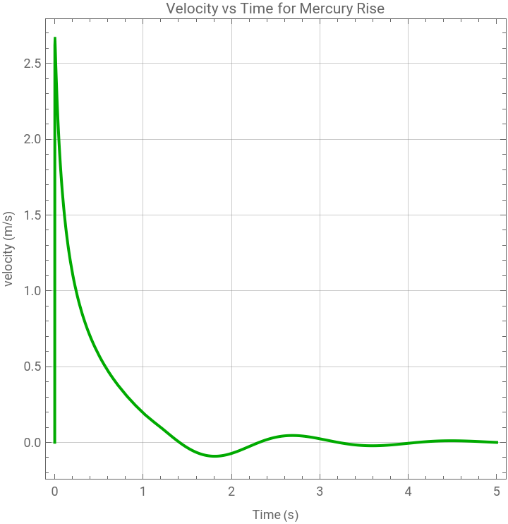
Plot[Evaluate[h'[t]/.sol],{t,0.0,5},Frame->True,FrameLabel->{"Time (s)","velocity (m/s)"},PlotLabel->"Velocity vs Time for Mercury Rise",GridLines->Automatic,PlotRange->All,PlotStyle->Darker@Green,AspectRatio->1]
Out[]=
In[]:=
Plot[Evaluate[-Ffric[t]]/.sol,{t,0.0,5},Frame->True,FrameLabel->{"Time (s)","visous damping force (N)"},PlotLabel->"viscous force vs Time for Mercury Rise",GridLines->Automatic,PlotRange->All,PlotStyle->Darker@Magenta,AspectRatio->1,PlotPoints->1000]
Out[]=