This is detailed the notebook to use with the linked YouTube video. All computation are rigorous and faithfully represent the unorthodox behavior of Cauchy distribution. We cover in-depth content to compare the given experiment with some variations, both numerically and symbolically. Also straightforward asymptotic results are given to help readers build up a big picture for the general behaviors of the distributions with divergent average.
Out[]=
Structure of the article
Structure of the article
◼
Follow the YouTube video to create simulation with Compile function
◼
Use symbolic and asymptotic result to verify the divergence of the average and variance
◼
Study a slight variant example
◼
Visualization on complex plane for some distributions
Experiment
Experiment
1
.Start with 2 balls in urn: 1 red and 1 blue
2
.If you pick a blue ball, terminate. If red, put the red ball back and add one red ball to the urn
3
.Repeat until you pick a blue ball
Find the average length of trials.
Simulation
Simulation
Rewrite the op’s python code and compile to native C. Assume 1 is the blue ball and all other numbers are red ball:
In[]:=
cf=Compile[{{n,_Integer}},Module[{round,balls,selected},Table[round=0;balls=2;selected=0;While[selected!=1,round++;selected=RandomInteger[{1,balls}];balls++];round,n]],CompilationTarget->"C"]
Out[]=
CompiledFunction


Benchmark: run 100K times
Benchmark: run 100K times
In[]:=
cf[100000];//AbsoluteTiming
Out[]=
{0.0312671,Null}
cf[100000]
Benchmark: run 10M times/This number jumps around
Benchmark: run 10M times/This number jumps around
In[]:=
Table[AssociationThread[{"Timing","Average trial length(10 million trials)"}->AbsoluteTiming[(N@Mean[cf[10^7]])]],{i,5}]//Dataset
Out[]=
The large variance in the computing time and result are from the nature of the distribution. Let’s compare the simulation with classic Bernoulli trial (no replenish of red ball)
In[]:=
(*balls++->ballsakanoadditionalredball*)cfB=Compile[{{n,_Integer}},Module[{round,balls,selected},Table[round=0;balls=2;selected=0;While[selected!=1,round++;selected=RandomInteger[{1,balls}];balls];round,n]],CompilationTarget->"C"]
Out[]=
CompiledFunction
In[]:=
Table[AssociationThread[{"Timing","Average trial length(10 million trials)"}->AbsoluteTiming[(N@Mean[cfB[10^7]])]],{i,5}]//Dataset
Out[]=
Several rounds of simulation with classic Bernoulli trials are very consistent.
We can also tabulate the measures and distribution for each run of simulation to build a summary for each round of repeating trials:
1
.mean value (average) and variance (spread-ness of the values)
2
.longest run
3
.distribution of the number of trials in each run
In[]:=
ds=Dataset[With[{res=cf[100000]},{<|"Average"->N@Mean[res],"Variance"->N@Variance[res],"Max"->Max[res],"Trial Length Distribution"->Histogram[res,{"Log",100},{"Log","Count"}]|>}]]
Out[]=
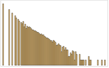
The histogram shows exactly how trial length distributed in each long run simulation.
Notice that some trial takes steps to finish in my test. Your number may vary after you run this multiple times.
Notice that some trial takes
~115310
Analytic solution
Analytic solution
Define the probability to terminate at n trials as :
p(n)
In[]:=
p[1]=1/2;
Similar to geometric distribution: requires (n-1) failures before the final successful trial:
In[]:=
p[n_]=FullSimplify,Assumptions->n∈PositiveIntegers
(n-1)!
(n+1)!
Out[]=
1
n+
2
n
Use telescoping to find the sum of p(n) is indeed 1
In[]:=
Sum[p[k],{k,1,Infinity}]
Out[]=
1
The average is
In[]:=
Sum[k*p[k],{k,1,n}]//FullSimplify
Out[]=
-1+HarmonicNumber[1+n]
This average value is divergent because that harmonic number diverges:
In[]:=
DiscreteLimit[HarmonicNumber[1+n],n->Infinity]
Out[]=
∞
Let’s do the same analysis for variance using definition. Use partial sum first:
In[]:=
var=With[{ek=Sum[k*p[k],{k,1,n}]//FullSimplify,ek2=Sum[k^2*p[k],{k,1,n}]//FullSimplify},ek2-ek^2]//FullSimplify
Out[]=
n+HarmonicNumber[1+n]-
2
HarmonicNumber[1+n]
In[]:=
DiscreteLimit[var,n->Infinity]
Out[]=
∞
Therefore no closed form and return unevaluated:
In[]:=
Expectation[x,x]
Out[]=
Expectationx,xProbabilityDistribution,x.,1,∞,1
1
x.+
2
x.
Visualize the distribution:
In[]:=
=ProbabilityDistribution"PDF",,{n,1,Infinity,1};
1
n+
2
n
In[]:=
Column@{DiscretePlot[PDF[,t]//Evaluate,{t,15},PlotLabel->"PDF"],DiscretePlot[CDF[,t]//Evaluate,{t,15},PlotLabel->"CDF"]}
Another experiment: Add two red balls instead of one
Another experiment: Add two red balls instead of one
1
.Start with 2 balls in urn: 1 red and 1 blue
2
.If you pick a blue ball, terminate. If red, put the red ball back and add TWO red ball to the urn
3
.Repeat until you pick a blue ball
Find the average length of trials.
I did some derivation and find the following PDF for the distribution:
Verify that it is indeed a valid discrete distribution by infinite summation:
Compute the partial expectation:
Because we add two red balls this time, this “expectation” should be “more divergent” than the previous one. Therefore the infinite sum does not exist either:
Visualize this compound special function:
Visualize on complex plane:
Therefore the expectation is of the order of
Utility
Utility
Generate the cover image
Generate the cover image
And put the
Exam the machine generated code. It should be “MainEvaluate” free.
CITE THIS NOTEBOOK
CITE THIS NOTEBOOK
Companion to "A Finite Game of Infinite Rounds": simulation of drawing balls from an urn
by Shenghui Yang
Wolfram Community, STAFF PICKS, September 6, 2023
https://community.wolfram.com/groups/-/m/t/3007279
by Shenghui Yang
Wolfram Community, STAFF PICKS, September 6, 2023
https://community.wolfram.com/groups/-/m/t/3007279