ABSTRACT (original article): Exactly solvable models in quantum many-body dynamics provide valuable insights into many interesting physical phenomena and serve as platforms for rigorously investigating fundamental theoretical questions. Nevertheless, they are extremely rare and existing solvable models and solution techniques have serious limitations. In this paper, we present a family of exactly solvable unitary circuits that model quantum many-body dynamics in discrete space and time. Unlike many previous solvable models, one can exactly compute the full quantum dynamics initialized from any matrix product state in this family of models. The time evolution of local observables and correlations, the linear growth of Rényi entanglement entropy, spatiotemporal correlations, and out-of-time-order correlations are all exactly computable. A key property of these models enabling the exact solution is that any time-evolved local operator is an exact matrix product operator with a finite bond dimension, even at arbitrarily long times, which we prove using the underlying ℂ*-(weak) Hopf algebra structure along with tensor network techniques. We lay down the general framework for construction and solution of this family of models, and give several explicit examples. In particular, we study in detail a model constructed out of a ℂ*-weak Hopf algebra that is very close to a Floquet version of the PXP model, and the exact results we obtain may shed light on the phenomenon of quantum many-body scars, and more generally, Floquet quantum dynamics in constrained systems. CITATION (original article): Zhiyuan Wang (2025), Hopf algebras and solvable unitary circuits, Phys. Rev. B 111, 104315. https://doi.org/10.1103/PhysRevB.111.104315
GitHub: https://github.com/lagrenge94/Hopf-algebras-and-solvable-unitary-circuits
GitHub: https://github.com/lagrenge94/Hopf-algebras-and-solvable-unitary-circuits
Constructing the tensors from algebraic data
Constructing the tensors from algebraic data
Load algebraic data from file; here R is the universal R - matrix which is not useful for this project
SetDirectory[NotebookDirectory[]];<<HAQCATools`;<<HATools`;<<TensorTools`;HAName="Fibonacci";{mul,Δ,η,ϵ,S,R,Rb}=LoadHA[HAName];{RepNames,CorepNames}
Out[]=
{{ρ2Map,ρ3Map},{V2,V3}}
Verify weak Hopf algebra axioms
VerifyWHAAxioms[mul,Δ,η,ϵ,S]
Out[]=
True
Check representation and corepresentation of
A
Fib
{CheckRep[ρ3Map,mul,η],CheckCorep[V3,Δ,ϵ]}//FullSimplify
Out[]=
{True,True}
Cosntruct {Ugate, ρRTensor, vRTensor, ηTensor, ϵTensor} using algebraic data via Eq . (2), and ρLTensor, vLTensor Via Eq . (E13) . (ρLTensor, vLTensor are not used in this code)
{Ugate,ρLTensor,ρRTensor,vLTensor,vRTensor,ηTensor,ϵTensor}=QCATensors[mul,Δ,η,ϵ,S,SparseArray@ρ3Map,SparseArray@V3];
Verify the first line of Eq . (1)
VerifyPentagon[Ugate,ρLTensor,ρRTensor,vLTensor,vRTensor,ηTensor,ϵTensor]//FullSimplify
Out[]=
{True,True}
Verify the second line of Eq . (1) . Then verifies the other 3 equations in Eq . (A20) . Note that since is only a WHA, only the latter is satisfied.
A
Fib
VerifyBoundaryηϵ[Ugate,ρLTensor,ρRTensor,vLTensor,vRTensor,ηTensor,ϵTensor]//FullSimplify
Out[]=
{False,True}
Compute local observables and correlations in quench dynamics
Compute local observables and correlations in quench dynamics
Prepare for numerical computations
ϕ=N;ζ=1,40;ζ=1
1+
5
2
ϕ
;Id=IdentityMatrix;{Ugate,ρLTensor,ρRTensor,vLTensor,vRTensor,ηTensor,ϵTensor}=N[{Ugate,ρLTensor,ρRTensor,vLTensor,vRTensor,ηTensor,ϵTensor}];(*Usethefollowinglinesforbetterprecision:*)(*$MinPrecision=40;ϕ=N1+
5
2
ϕ
;{Ugate,ρLTensor,ρRTensor,vLTensor,vRTensor,ηTensor,ϵTensor}=N[QCATensors[mul,Δ,η,ϵ,S,SparseArray@ρ3Map,SparseArray@V3],40];*)Define the initial product state
Ψ33=N[SparseArray/@ProductStateMPS[{0,0,1},{0,0,1}]];(*forbetterprecision:*)(*Ψ33=N[SparseArray/@ProductStateMPS[{0,0,1},{0,0,1}],40];*){χL,χR,ψρ,ψv}=Ψ33;
Define local observables and correlations functions to compute in quench dynamics
Corr33[A_,B_,x_,t_]:=Corr[A,B,Ψ33,x,t,ρRTensor,vRTensor,ηTensor,ϵTensor];Observable33[A_,t_]:=If[Mod[2t,2]0,Corr33[A,Id[3],0,t],Corr33[Id[3],A,0,t]];O32[t_]:=If[Mod[2t,2]0,Corr33[el[3,3,3],el[2,2,3],0,t],Corr33[el[3,3,3],el[2,2,3],0,t+1/2]];O3321[t_]:=If[Mod[2t,2]0,2Re[Corr33[el[3,2,3],el[3,1,3],0,t]],2Corr33[el[2,2,3],el[1,1,3],0,t+1/2]-2Corr33[el[3,3,3],el[3,3,3],0,t+1/2]+2Re@Corr33[el[3,2,3],el[3,1,3],0,t+1/2]];
3
ζ
3
ζ
6
ζ
In[]:=
<<MaTeX`;
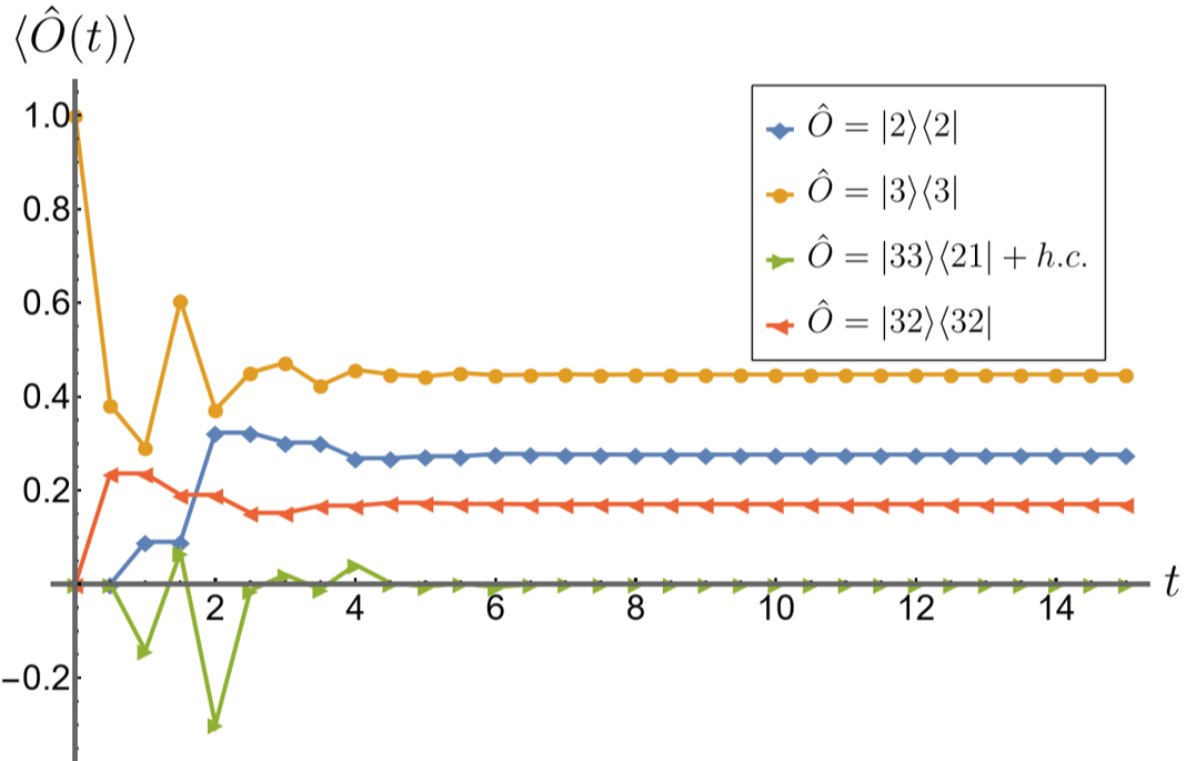
Reproduce Fig .3
DiscretePlot[{Observable33[el[2,2,3],t],Observable33[el[3,3,3],t],O3321[t],O32[t]},{t,0,15,1/2},PlotRangeAll,PlotStyleAbsoluteThickness[3],PlotLegendsPlaced[LineLegend[{MaTeX["\\hat{O}=|2\\rangle\\langle 2|",Magnification2.],MaTeX["\\hat{O}=|3\\rangle\\langle 3|",Magnification2.],MaTeX["\\hat{O}=|33\\rangle\\langle 21|+h.c.",Magnification2.],MaTeX["\\hat{O}=|32\\rangle\\langle 32|",Magnification2.]},LegendFunctionFramed],{0.8,0.79}],AxesLabel{MaTeX["t",Magnification2.8],MaTeX["\\langle\\hat{O}(t)\\rangle",Magnification2.8]},TicksStyleDirective[Black,Thick,24],FillingNone,JoinedTrue,(*PlotMarkersNone,*)(*PlotMarkers{"▲","■"},*)PlotMarkers{{"◆",20},{"●",16},{"▶",20},{"◀",20}},AxesStyleAbsoluteThickness[3.5]]
Out[]=
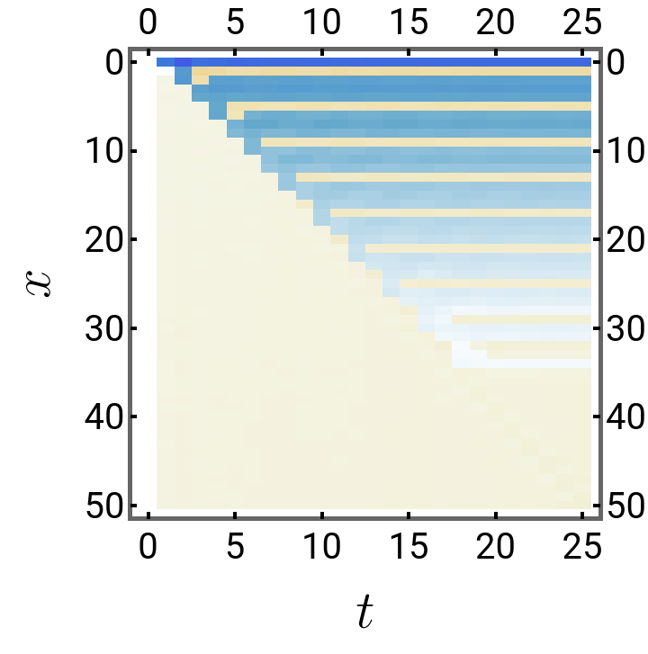
Plot correlation function (x,t) defined in Eq . (69)
ij
W
WPlot[i_,j_,xRange_]:=Module[{W,WData},(*W[x_,t_]:=If[x>2t,0,Corr33[el[i,i,3],el[j,j,3],x,t]-Corr33[el[i,i,3],Id[3],x,t]*Corr33[Id[3],el[j,j,3],x,t]];*)W[x_,t_]:=Corr33[el[i,i,3],el[j,j,3],x,t]-Corr33[el[i,i,3],Id[3],x,t]*Corr33[Id[3],el[j,j,3],x,t];WData=Table[{x,t,W[x,t]},{x,0,xRange},{t,0,xRange/2}];MatrixPlot[Reverse@WData[[All,All,3]],AspectRatio1,DataRange{{0,xRange/2},{0,xRange}},FrameLabel{MaTeX["x",Magnification2.5],MaTeX["t",Magnification2.5]},FrameTicksStyleDirective[Black,Thick,20],FrameStyleAbsoluteThickness[2.5],DataReversedTrue]];
Reproduce Fig .4
Note : to exactly reproduce Fig .4, one need to use higher numerical precisions in earlier steps
Note : to exactly reproduce Fig .4, one need to use higher numerical precisions in earlier steps
WPlot[2,2,50]
Out[]=
Compute Renyi Entanglement entropy in quench dynamics
Compute Renyi Entanglement entropy in quench dynamics
Compute the transfer matrices needed for Renyi entanglement entropy calculations
Compute the Renyi Entanglement entropy for small subsystem, and reproduce the first plot in Fig .5.
Compute the Renyi Entanglement entropy for large subsystem and small index α, and reproduce the second plot in Fig .5 . This may take up to an hour
Compute the Renyi Entanglement entropy for a semiinfinite half chain, and reproduce the last plot in Fig .5.
Verify finite system revival time
Verify finite system revival time
Apply ρfund and vfund to the canonical element via Eq . (A36)
So we conclude that the canonical element has order n = 5
Now compute numerically the revival time for small system sizes L = 2, 3, 4
For L = 2, revival time is n L = 10
For L = 3, revival time is n L = 15
For L = 4, revival time is n L = 20
CITE THIS NOTEBOOK
CITE THIS NOTEBOOK
Hopf algebras and solvable unitary circuits
by Zhiyuan Wang
Wolfram Community, STAFF PICKS, May 27, 2025
https://community.wolfram.com/groups/-/m/t/3469749
by Zhiyuan Wang
Wolfram Community, STAFF PICKS, May 27, 2025
https://community.wolfram.com/groups/-/m/t/3469749