Trained neural nets generally store semantic information about the data that they operate on. This is typically referred to as an “embedding space”, which is where similarities and differences between outputs can be derived.
In the context of 3D geometry, the embedding space differs depending on the encoding method used. This computational essay explores the embedding space of various neural nets that reconstruct 3D geometrical shapes in various forms, including discrete voxel grids and continuous signed distance functions.
In the context of 3D geometry, the embedding space differs depending on the encoding method used. This computational essay explores the embedding space of various neural nets that reconstruct 3D geometrical shapes in various forms, including discrete voxel grids and continuous signed distance functions.
Global Initializations
Global Initializations
Introduction
Introduction
If you told a past version of myself that one day I’d be working on a project involving generative AI, I wouldn’t have believed you. At my current stage in life, I am just over a year into a Master of Fine Arts program in Digital Media. As part of this work, I focus on real-time computer graphics, but I am also in a cohort with game designers, animators, and 3D modelers, among others. My perception of generative AI in most contexts has been primarily negative.
After starting the Wolfram Summer Research Institute, my perspective shifted. I saw that the questions surrounding generative AI were much more nuanced than I initially realized. In fact, there are some interesting problems to solve when it comes to creating, designing, and training large scale neural nets. While I continue to stand behind the idea that generative art should never replace real human artists, I cannot deny the curiosity that arises when exploring neural net applications.
In Stephen Wolfram's blog titled “Generative AI Space and the Mental Imagery of Alien Minds”, he writes that recent advancements in neural nets and generative AI can give us a perspective on how a non-human mind forms mental images. The following essay aims to extend this concept and apply it to 3D geometry by presenting two methods for encoding geometric data in the Wolfram Language. It also briefly explores the “embedding space” of neural nets trained on 3D data by morphing between shapes and observing the results.
After starting the Wolfram Summer Research Institute, my perspective shifted. I saw that the questions surrounding generative AI were much more nuanced than I initially realized. In fact, there are some interesting problems to solve when it comes to creating, designing, and training large scale neural nets. While I continue to stand behind the idea that generative art should never replace real human artists, I cannot deny the curiosity that arises when exploring neural net applications.
In Stephen Wolfram's blog titled “Generative AI Space and the Mental Imagery of Alien Minds”, he writes that recent advancements in neural nets and generative AI can give us a perspective on how a non-human mind forms mental images. The following essay aims to extend this concept and apply it to 3D geometry by presenting two methods for encoding geometric data in the Wolfram Language. It also briefly explores the “embedding space” of neural nets trained on 3D data by morphing between shapes and observing the results.
Background
Background
Neural Net Embedding Space
Neural Net Embedding Space
The concept of embedding space refers to a neural net’s semantic understanding of the data type it operates on. For example, consider asking a generative AI model to create the following two images from a text input:
Out[]=
,
Cat in a party hat |

Dog in a party hat |
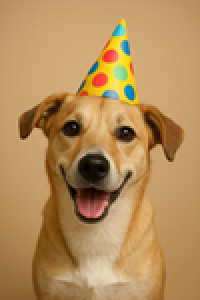
The only difference in input is the word “dog” and the word “cat”; this implies that there is a semantic difference between the two inputs resulting in a clearly different output. For words and images, this is relatively intuitive. But how does the concept of “embedding space” apply to more abstract data types, such as 3D geometry?
3D Geometry Encoding
3D Geometry Encoding
To start exploring this question, we have to start by finding a way to encode geometric data so that a neural net can process it. One key complication is that there are several ways that 3D geometry can be represented. Shapes can be rendered through polygonal meshes, discrete grid structures, and parametric functions.
A sphere represented in 3 ways:
(1. A triangle-based mesh; 2. A grid-based Image3D object; 3. A parametric 3D plot)
(1. A triangle-based mesh; 2. A grid-based Image3D object; 3. A parametric 3D plot)
Out[]=
 ,
, ,
,
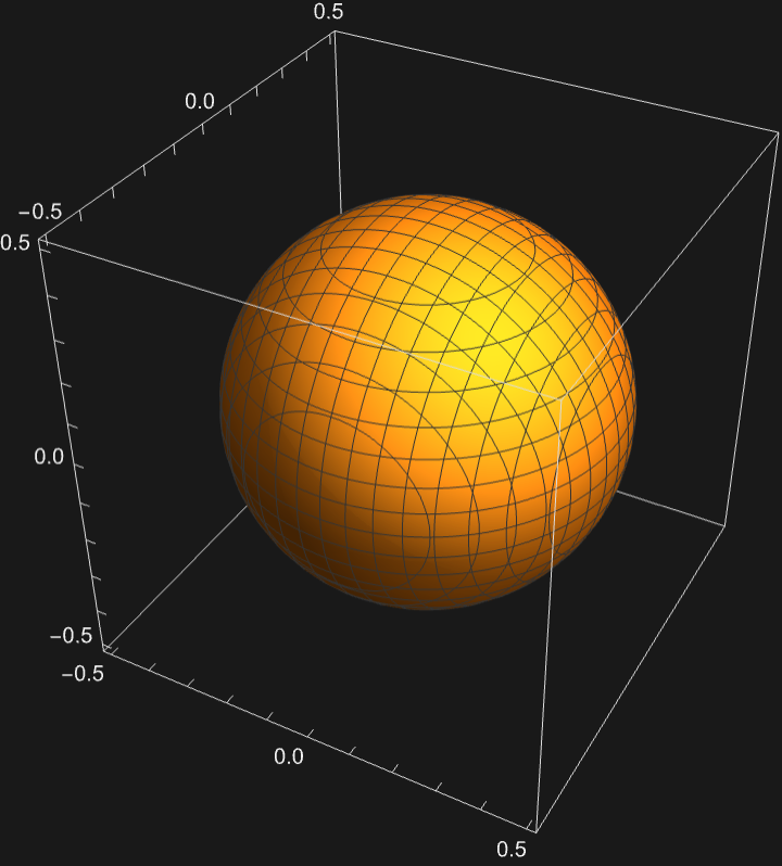
Of the existing models in the Wolfram Neural Net Repository, relatively few are designed to operate on 3D geometry. The models primarily accept text, audio, and 2D images as input, and produce a similar output. As a result, it can be challenging to approach working with 3D geometry and neural nets in the Wolfram Language. The following encoding methods presented aim to provide the starting points for future work involving machine learning and 3D shape representations.
Encoding Methods
Encoding Methods
Method 1 - Voxel Grid Encoding
Method 1 - Voxel Grid Encoding
Introduction
Introduction
Voxels are a discrete data structure that can be used to represent 3D geometry. Similar to an image storing a 2D array of pixels, voxels represent a 3D array of values that describe the form of some shape.
Drawing a voxel sphere:
Out[]=

One key consideration when using this shape representation is “voxel resolution”. A voxel grid takes up n x n x n space, where n is 32 in this case. A higher value leads to better shape definition at the cost of more memory usage and more neural net training time.
Voxel octahedron of varying resolutions:
Out[]=
,
,
 |
1. n = 16 |
 |
2. n = 32 |
 |
3. n = 64 |
This poses an interesting challenge when training a model. Consider the following shape set:
A set of distinct, yet visually similar 16x16x16 shapes:
Out[]=
,
,
 |
1. Sphere |
 |
2. Dodecahedron |
 |
3. Icosahedron |
At low resolutions, shapes start to become indistinguishable from one another. It is important to use an appropriate resolution, ideally at least n=32 when using voxel shape representations.
Data Generation
Data Generation
Conveniently, once a resolution has been established for a dataset, every voxel shape will have the same dimensions.
The dataset used for training uses the following 8 shape classes:
Out[]=
,
,
,
,
,
,
,
 |
1. Sphere |
 |
2. Cube |
 |
3. Cone |
 |
4. Octahedron |
 |
5. Dodecahedron |
 |
6. Cylinder |
 |
7. Pyramid |
 |
8. Icosahedron |
The training data we are using to train the model provides a specific shape as input and the same shape as output. The end goal is for the model to be able to reconstruct a given shape. We can then use the intermediate layer as the “embedding space” to begin exploring relationships between shape classes.
Creating the dataset with each shape class as input and output:
In[]:=
voxelShapeData=Join[spheres,cubes,cones,octahedrons,dodecahedrons,icosahedrons,cylinders,pyramids];voxelTrainingData=Thread[voxelShapeData->voxelShapeData];
Training the Network
Training the Network
A convolutional neural network is a kind of neural net that works well on extracting features from evenly spaced data types. One of the simplest applications of this kind of neural net is recognizing handwritten digits. The consistent dimensions of a voxel grid work in our benefit once again, making convolution a straightforward operation to apply to a voxel grid. The process of encoding breaks down the 32x32x32 grid into a 64 dimensional embedding layer, which is then used for reconstruction.
The net chain used to encode the voxel grid is as follows:
Out[]=
NetChain

Training the net using 100 rounds:
Extracting the net from the results:
Shape Reconstruction
Shape Reconstruction
After training, we can reconstruct shapes by using the layers as an encoder / decoder pair. The convolution layers are the “encoder” and the reconstruction layers are the “decoder”.
Extracting the encoder and decoder:
Shape Reconstruction:
For some shape classes, such as the cylinder and dodecahedron, the neural net performed very well. However, for “pointier” classes, such as the pyramid, it performed quite poorly.
One of the best ways to visualize a dataset in the Wolfram Language is to use a feature extractor. We can use the encoder extracted earlier to reduce the 64 dimensional embedding layer down to a 3D coordinate plot.
Building a feature plot from the encoder:
We can see some interesting groupings for the shape classes. The cylinder and dodecahedron were two shapes that were reconstructed with the highest accuracy, while also having a distinct feature of having large, flat areas on their sides. Two poorly reconstructed shapes, the pyramid and cone, are also grouped together. The icosahedron was rounded out during reconstruction, and appears close to the sphere.
These groupings imply that there is a distinct feature set for various shape classes. While the reconstruction is not perfect in all cases, we can still visualize a seemingly meaningful relationship between the neural net’s encoding for each shape.
These groupings imply that there is a distinct feature set for various shape classes. While the reconstruction is not perfect in all cases, we can still visualize a seemingly meaningful relationship between the neural net’s encoding for each shape.
Shape Morphing
Shape Morphing
Another interesting observation we can make from the feature plot is the distance between different shapes. For example, the sphere and cylinder are quite far apart. How can we visualize the “in-between” space for these two shapes?
Displaying the “in-between” steps of a sphere and a cylinder:
When morphing between a sphere and a cylinder, the net appears to take a reasonable series of steps without too much noise in the middle. From this, we should expect to be able to map a relatively linear path in our feature graph to get from “sphere space” to “cylinder space”. We can try this out by mapping the intermediate shapes in another feature plot.
Creating a 3D space plot for morphing shapes:
While not perfectly linear, there is a reasonable path to get from “sphere space” to “cylinder space’, which is why we see such clear results when morphing between them. We can overlay this path onto our original feature graph with all 8 shape classes.
Showing “sphere” to “cylinder” on our original feature graph:
Method Summary
Method Summary
Voxel shape representation works as an encoding method for 3D geometry, with some caveats. It is necessary to use a resolution high enough to differentiate between shape classes. Additionally, shape classes with “pointier” features are more susceptible to noise, leading to less accurate reconstructions. However, with larger datasets and more training, it may be possible to mitigate the frequency of noise.
Method 2 - Signed Distance Functions
Method 2 - Signed Distance Functions
Introduction
Introduction
Signed distance functions (SDFs) provide a continuous, parametric way of describing a geometric shape. By providing some 3D point {x, y, z}, the function outputs the distance to the surface of the shape we want to represent.
We can render the SDFs of some primitives with a contour plot:
Data Generation
Data Generation
In order to encode an SDF for use in a neural net, we need to generate a list of points paired with the expected output. The input / output pairs are the data we will use to train the net.
Start by generating the “inputs”, which will be used for each function:
Map the inputs over each function to generate the expected outputs:
In addition to the input / output pairs, we also need a parameter that lets the neural net know which function to evaluate. This is to avoid needing a unique net for each shape we want to generate. This means that the final input to the neural net is a 4D vector of the form:
Where n is the index of the specific function we are evaluating, and x, y & z are the inputs to that function. The neural net then outputs a single real number.
Training the Network
Training the Network
We can use a much simpler neural network for encoding signed distance functions.
The net chain for signed distance function encoding:
Training the net:
Extracting the trained net from the results:
Shape Reconstruction
Shape Reconstruction
After training, we can reconstruct shapes by evaluating the neural net on a given set a points and plotting the results.
Plotting SDFs and their trained versions:
With just a few minutes of training, the net is able to reconstruct a few primitives reasonably well. It primarily struggles to recreate sharp edges, such as those present on a cube and a cylinder.
Shape Morphing
Shape Morphing
What happens in the “in-between” space of two shapes when using this method? Recall that for the voxel-based approach, we were able to plot a feature graph to visualize the relationship between different shape classes. In this case, the neural net’s output is a single number, rather than a fully reconstructed shape.
One way that we can explore intermediate shape space is by providing an index we never trained the net on. In this case, we can provide the values between 0 and 1 and see how the output changes.
One way that we can explore intermediate shape space is by providing an index we never trained the net on. In this case, we can provide the values between 0 and 1 and see how the output changes.
Interpolating between a sphere and cube:
Shape Extrapolation
Shape Extrapolation
We can also see what happens “outside” of the networks learned inputs by using a negative index, or one outside of the specified range.
Shapes generated outside of the net’s learned shape range:
The net is able to interpolate between shapes reasonably well, resulting in a sort of balloon-like appearance when moving from one shape to another. Extrapolating can lead to some visually distinct results, but they don’t take the form of any of the trained shapes we gave to the net.
Method Summary
Method Summary
Training a net using signed distance functions is a feasible approach, as it able to provide a form of shape reconstruction with just a few minutes of training. The primary considerations are the level of detail on the input shapes and the need for extrapolation. Sharp corners and fine details can be lost in training, and extrapolation may not yield predictable results.
Concluding Remarks
Concluding Remarks
Despite the irregularities of 3D geometrical data, it is possible to train neural nets to reconstruct shapes. Results vary based on the data type chosen. For discrete voxel grids, the memory requirements are quite large for high resolution datasets, yet it is easier to derive a unique feature set for each shape class. For continuous signed distance functions, training is relatively quick, but finer details can be lost.
In addition to reconstruction, these methods provide a means to explore the relationship between distinct shapes. When interpolating between shapes rendered with voxels, we can define a clear path to get from one shape to another. When doing the same for signed distance functions, we also get sensible in-between steps and predictable visual results. The same cannot be said for extrapolation; results when extrapolating outside of the net’s learned shape range tended to be noisy and unpredictable, albeit visually intriguing,
In addition to reconstruction, these methods provide a means to explore the relationship between distinct shapes. When interpolating between shapes rendered with voxels, we can define a clear path to get from one shape to another. When doing the same for signed distance functions, we also get sensible in-between steps and predictable visual results. The same cannot be said for extrapolation; results when extrapolating outside of the net’s learned shape range tended to be noisy and unpredictable, albeit visually intriguing,
Future Work
Future Work
The methods presented here show promising potential for future Wolfram Language projects that combine machine learning and 3D geometrical data. Adding more shape classes and using a voxel resolution of 64 would likely lead to more robust results when using the voxel grid encoding approach. Using a larger domain (beyond -1 and 1) and a larger point set would likely help to mitigate the feature loss for signed distance functions. The neural net architecture could also be altered to have more learned layers.
It is worth mentioning that there are existing techniques not mentioned in this essay that operate on the edges of a triangle-based mesh that could work in the Wolfram Language. Two standouts are the convolutional approach titled MeshCNN and the transformer based approach titled MeshGPT. These approaches are much less straightforward in regards to their implementation details, but would likely prove incredibly useful if done successfully.
Future work could also operate on the practical applications of 3D shape encoding. The neural nets presented were never trained on classification, only on reconstruction. Despite this, it seemed that the nets created their own vocabulary for representing different shape types. In the net trained on voxels, shapes with flat edges were grouped together, separate from pointy or smooth shapes. Another key finding is that certain shapes were reconstructed very well, while others were not. The ability for a net to properly reconstruct a given shape class could provide useful information in several areas involving the use of 3D geometry, such as 3D printing, or in medical fields where 3D images are used.
It is worth mentioning that there are existing techniques not mentioned in this essay that operate on the edges of a triangle-based mesh that could work in the Wolfram Language. Two standouts are the convolutional approach titled MeshCNN and the transformer based approach titled MeshGPT. These approaches are much less straightforward in regards to their implementation details, but would likely prove incredibly useful if done successfully.
Future work could also operate on the practical applications of 3D shape encoding. The neural nets presented were never trained on classification, only on reconstruction. Despite this, it seemed that the nets created their own vocabulary for representing different shape types. In the net trained on voxels, shapes with flat edges were grouped together, separate from pointy or smooth shapes. Another key finding is that certain shapes were reconstructed very well, while others were not. The ability for a net to properly reconstruct a given shape class could provide useful information in several areas involving the use of 3D geometry, such as 3D printing, or in medical fields where 3D images are used.
Acknowledgments
Acknowledgments
I would like to start by thanking Allen & Julia Gary for introducing me to the Wolfram Summer Research Institute, and for providing the support for me to attend. I would also like to thank my project mentor, Christian Pasquel, and the other members of my group, Ahmet Erhan, Enrico Bottazzi, and Mohamed AlBegaowe for their support throughout the entire program. Additional thanks to Nora Popescu and Faizon Zaman for reading early drafts and providing feedback. Finally, thank you to Stephen Wolfram for the project suggestion.
References
References
1
.J. Park et al., (2019), “DeepSDF: Learning Continuous Signed Distance Functions for Shape Representation,” Proceedings of the IEEE/CVF Conference on Computer Vision and Pattern Recognition (CVPR), pp. 165-174. https://openaccess.thecvf.com/content_CVPR_2019/html/Park_DeepSDF_Learning_Continuous_Signed_Distance_Functions_for_Shape_Representation_CVPR_2019_paper.html.
AI Disclosure
AI Disclosure
The following generative AI tools were used in this project: Claude Opus 4.8, Google AI Overview. They were used for brainstorming, documentation retrieval, and debugging. All code and written content was reviewed, understood and approved by the author.
CITE THIS NOTEBOOK
CITE THIS NOTEBOOK
Neural Net Encoding Methods for 3D Geometry
by Caden Lafollette
Wolfram Community, STAFF PICKS, July 16, 2026
https://community.wolfram.com/groups/-/m/t/3762308
by Caden Lafollette
Wolfram Community, STAFF PICKS, July 16, 2026
https://community.wolfram.com/groups/-/m/t/3762308