We analyzes a solute extraction process. A raffinate stream with volumetric flow containing an unwanted solute enters a five-stage extraction cascade that is connected to a tank holding the extraction solvent.
The solvent container is modeled as a perfectly mixed tank such that the solute composition leaving the tank at any time is the same as the composition in the tank at that time.
This problem was solved analytically by Ugo Lelli [1].
Here, a numerical solution using Mathematica is given that lets you examine how two key parameters for the extraction process influence the system performance.
You can see the effect of varying different values of the solvent container residence time (expressed as a dimensionless parameter ) and the dimensionless parameter (related to the volumetric flow rates and in the raffinate and extract phases).
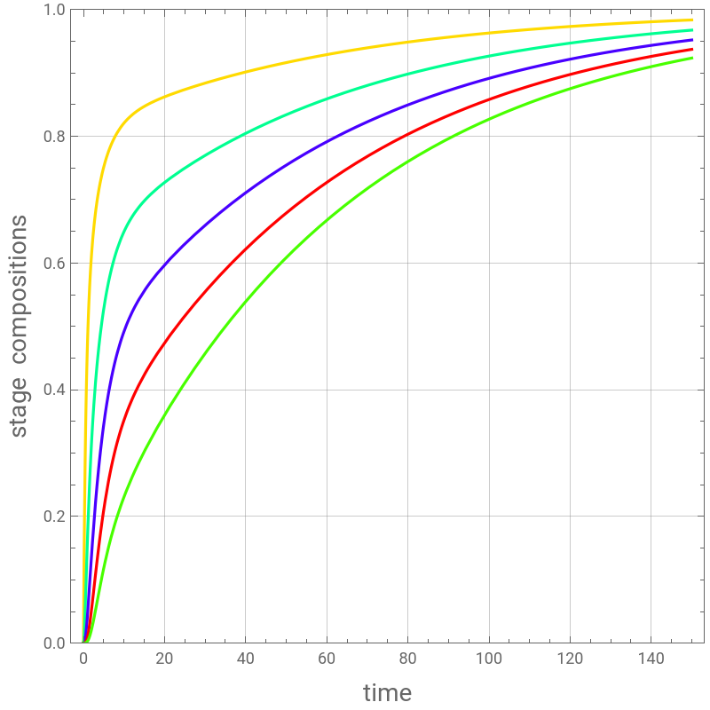
We show how the equilibrium composition (in the raffinate phase) of each stage in the cascade varies with extraction time, expressed in terms of the dimensionless variable. At the start =0, there is no solute in the solvent stream and thus ==0. Then at =, the raffinate stream has a step change in solute concentration ()=1.
For very large values of the residence time or dimensionless parameter, we get the usual equilibrium cascade behavior without recycle and (t)≈0 for all and . In contrast, for small values of residence time (or ), solvent saturation is observed at large values of the dimensionless time .
For very large values of h, we get the usual cascade without recycle problem . For small values of h and large times, we get solvent saturation .
Finally, we extend Lelli’ s work by considering the case of a plug flow container.
R
The solvent container is modeled as a perfectly mixed tank such that the solute composition leaving the tank at any time is the same as the composition in the tank at that time.
This problem was solved analytically by Ugo Lelli [1].
Here, a numerical solution using Mathematica is given that lets you examine how two key parameters for the extraction process influence the system performance.
You can see the effect of varying different values of the solvent container residence time
τ
h
λ=R/(mE)
R
E
We show how the equilibrium composition (in the raffinate phase) of each stage in the cascade varies with extraction time, expressed in terms of the dimensionless variable
*
t
*
t
Y
1
Y
6
*
t
+
0
X
1
+
0
For very large values of the residence time or dimensionless parameter
h
Y
6
t
h=100000
h
*
t
For very large values of h, we get the usual cascade without recycle problem . For small values of h and large times, we get solvent saturation .
Finally, we extend Lelli’ s work by considering the case of a plug flow container.
Theoretical Background
Theoretical Background
A material balance over the solute phase for an arbitrary stage is:=R-R-, =E-E+,where and are the stage holdup volumes expressed in for the raffinate and extract phases; and are the solute mass fractions in the raffinate and extract phases leaving the stage, respectively; and are the volumetric flow rates for the extract and raffinate phases expressed in /min; and is the volumetric rate of solute that is transferred between phases at the stage. If equilibrium is established at each stage so that =m, the solute material balances can be combined to give a single equation for the change in mass fraction of solute in the raffinate at the stage: .For computational purposes it is convenient to work with the dimensionless form of this equation, which for the stage is given by:=λ+-(1+λ),where is the dimensionless solute composition given by =/(t=0). For the dilute system approximation to hold, we require that (t=0)≪1. The specified dimensionless inlet composition of the raffinate stream for >0 is ()=1. The dimensionless time is defined as =tEm/(+m), while the flow rate ratio parameter is given by . Finally, the dynamic behavior of the solvent tank (when we assume a perfectly mixed tank), is governed by:, (0)=0, or equivalently, , (0)=0,where the dimensionless parameter and is the residence time of the solvent tank with volume .
n
H
R
d
X
n
dt
X
n-1
X
n
Q
n
H
E
d
Y
n
dt
Y
n+1
Y
n
Q
n
H
R
H
E
3
m
X
n
Y
n
th
n
E
R
3
m
Q
n
th
n
Y
n
X
n
th
n
(+m)=R-(R+mE)+mE
H
R
H
E
d
X
n
dt
X
n-1
X
n
X
n+1
th
n
*
X
n
*
t
*
X
n-1
*
X
n+1
*
X
n
*
X
n
*
X
n
X
n
X
0
X
0
*
t
*
X
0
*
t
*
t
H
R
H
E
λ=R/(Em)
h=-
*
Y
6
*
t
*
Y
1
*
Y
6
*
Y
6
h=-
*
X
6
*
t
*
X
1
*
X
6
*
X
6
h=Vm/(+m)=τEm/(+m)
H
R
H
E
H
R
H
E
τ=V/E
V
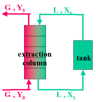
First case: Solvent tank is a perfectly mixed container.
λ is proportional to the equilibrium constant. h depends on tank volume
λ is proportional to the equilibrium constant. h depends on tank volume
Plotting the five stages dimensionless compositions (,,,,) versus time for λ=1 and h=50.
*
X
1
*
X
2
*
X
3
*
X
4
*
X
5
In[]:=
λ=1;
In[]:=
X
0
In[]:=
h=50;
In[]:=
sol1=NDSolve[{[t]-(1+λ)[t]+λ[t]D[[t],{t,1}],[t]-(1+λ)[t]+λ[t]D[[t],{t,1}],[t]-(1+λ)[t]+λ[t]D[[t],{t,1}],[t]-(1+λ)[t]+λ[t]D[[t],{t,1}],[t]-(1+λ)[t]+λ[t]D[[t],{t,1}],hD[[t],{t,1}]([t]-[t]),[0]0,[0]0,[0]0,[0]0,[0]0,[0]0},{[t],[t],[t],[t],[t],[t]},{t,0,150}]
X
6
X
5
X
4
X
5
X
5
X
4
X
3
X
4
X
4
X
3
X
2
X
3
X
3
X
2
X
1
X
2
X
2
X
1
X
0
X
1
X
6
X
1
X
6
X
1
X
2
X
3
X
4
X
5
X
6
X
1
X
2
X
3
X
4
X
5
X
6
Out[]=
[t]InterpolatingFunction[t],[t]InterpolatingFunction[t],[t]InterpolatingFunction[t],[t]InterpolatingFunction[t],[t]InterpolatingFunction[t],[t]InterpolatingFunction[t]
X
1


X
2

X
3

X
4

X
5

X
6

In[]:=
Plot[Evaluate[{[t],[t],[t],[t],[t]}/.sol1],{t,0,150},PlotRange{0,1},PlotStyleTable[Hue[(2i-1)/7],{i,1,5}],Frame->True,GridLines->Automatic,FrameLabel->{Style["time",14],Style["stage compositions",14]},AspectRatio->1,ImageSize->400{1,1}]
X
1
X
2
X
3
X
4
X
5
Out[]=
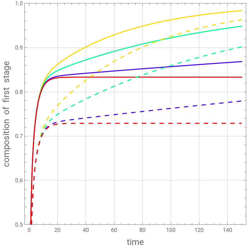
Plotting the first stage dimensionless composition () versus time for λ=1 (solid line) and 0.8 (dashed line).
h is set equal to 50, 100, 500 and 10^10.
We obtain the case without recycle for h very large (i.e. 10^10).
For h small, we reach solvent saturation (=1) after a short period of time.
*
X
1
h is set equal to 50, 100, 500 and 10^10.
We obtain the case without recycle for h very large (i.e. 10^10).
For h small, we reach solvent saturation (
*
X
1
In[]:=
sol[h_,λ_]:=NDSolve[{[t]-(1+λ)[t]+λ[t]D[[t],{t,1}],[t]-(1+λ)[t]+λ[t]D[[t],{t,1}],[t]-(1+λ)[t]+λ[t]D[[t],{t,1}],[t]-(1+λ)[t]+λ[t]D[[t],{t,1}],[t]-(1+λ)[t]+λ[t]D[[t],{t,1}],hD[[t],{t,1}]([t]-[t]),[0]0,[0]0,[0]0,[0]0,[0]0,[0]0},{[t],[t],[t],[t],[t],[t]},{t,0,150}]
X
6
X
5
X
4
X
5
X
5
X
4
X
3
X
4
X
4
X
3
X
2
X
3
X
3
X
2
X
1
X
2
X
2
X
1
X
0
X
1
X
6
X
1
X
6
X
1
X
2
X
3
X
4
X
5
X
6
X
1
X
2
X
3
X
4
X
5
X
6
In[]:=
plt1=Plot[Evaluate[{[t]/.sol[50,1],[t]/.sol[100,1],[t]/.sol[500,1],[t]/.sol[10^10,1]}],{t,0,150},PlotRange{0.5,1},PlotStyleTable[Hue[(2i-1)/7],{i,1,5}],FrameTrue,GridLines->Automatic];
X
1
X
1
X
1
X
1
In[]:=
plt2=Plot[Evaluate[{[t]/.sol[50,0.8],[t]/.sol[100,0.8],[t]/.sol[500,0.8],[t]/.sol[10^10,0.8]}],{t,0,150},PlotRange{0.5,1},PlotStyle{{Dashing[{0.02}],Hue[1/7]},{Dashing[{0.02}],Hue[3/7]},{Dashing[{0.02}],Hue[5/7]},{Dashing[{0.02}],Hue[7/7]}},FrameTrue,GridLines->Automatic];
X
1
X
1
X
1
X
1
In[]:=
Show[plt1,plt2,FrameLabel->{Style["time",14],Style["composition of first stage",14]},AspectRatio->1,ImageSize->400{1,1}]
Out[]=
Second case: Solvent tank is a plug flow container.
λ is proportional to the equilibrium constant. h depends on tank volume
λ is proportional to the equilibrium constant. h depends on tank volume
Plotting the dimensionless composition (, , , , ) versus time () for λ=1 and h=50.
*
X
1
*
X
2
*
X
3
*
X
4
*
X
5
150>=>=0
*
t
In[]:=
λ=1;
In[]:=
X
0
In[]:=
h=50;
In[]:=
X
6
In[]:=
sol2=NDSolve[{[t]-(1+λ)[t]+λ[t]D[[t],{t,1}],[t]-(1+λ)[t]+λ[t]D[[t],{t,1}],[t]-(1+λ)[t]+λ[t]D[[t],{t,1}],[t]-(1+λ)[t]+λ[t]D[[t],{t,1}],[t]-(1+λ)[t]+λ[t]D[[t],{t,1}],[0]0,[0]0,[0]0,[0]0,[0]0},{[t],[t],[t],[t],[t]},{t,0,50}]
X
6
X
5
X
4
X
5
X
5
X
4
X
3
X
4
X
4
X
3
X
2
X
3
X
3
X
2
X
1
X
2
X
2
X
1
X
0
X
1
X
1
X
2
X
3
X
4
X
5
X
1
X
2
X
3
X
4
X
5
Out[]=
[t]InterpolatingFunction[t],[t]InterpolatingFunction[t],[t]InterpolatingFunction[t],[t]InterpolatingFunction[t],[t]InterpolatingFunction[t]
X
1

X
2

X
3

X
4

X
5

In[]:=
Show[plt3,plt4,plt5,PlotRange-> All]
References
References
[1] U. Lelli, Annali di Chimica, 56, 1966 pp. 113–125.
[2] J. Ingham, I. J. Dunn, E. Heinzle, and J. E. Prenosil, Chemical Engineering Dynamics, 2nd ed., Weinheim, Germany: Wiley-VCH, 2000.
[2] J. Ingham, I. J. Dunn, E. Heinzle, and J. E. Prenosil, Chemical Engineering Dynamics, 2nd ed., Weinheim, Germany: Wiley-VCH, 2000.
CITE THIS NOTEBOOK
CITE THIS NOTEBOOK
Dynamics of a Five Equilibrium Stages Extraction Cascade with Solvent Recycle
by Housam Binous and Ahmed Bellagi
Wolfram Community, STAFF PICKS, November 4, 2023
https://community.wolfram.com/groups/-/m/t/3060194
by Housam Binous and Ahmed Bellagi
Wolfram Community, STAFF PICKS, November 4, 2023
https://community.wolfram.com/groups/-/m/t/3060194