ABSTRACT (original article): This work surveys the use of directed weighted graphs in conducting comparative static analyses. The paper discusses the implementation of a computer-aided process for building spreadsheet-based graph models for inter- and intra-regional financial flows. The graph-theoretic techniques are programmed to enable the interactive visualization and analysis of financial data using Wolfram technologies (i.e., Mathematica software v. 11.3 or later, Wolfram player v. 12 or later). The paper describes the workflow for several interactive visualizations applicable to financial networks. The author provides four programs, written in the Wolfram language, that customize input–output financial models by combining the Manipulate command with built-in Mathematica functions and functions of the IGraph package (IGraph/M). The study is a tutorial article for the generation of a suite of visual schemes that provide patterns, practices, and roadmaps of the financial markets across the globe. CITATION (original article): Tsilika, K. (2024). A Mathematica-Based Interface for the Exploration of Inter- and Intra-Regional Financial Flows. Mathematics, 12(6), 877. https://doi.org/10.3390/math12060877
This file shows how to use some of Mathematica’ s built - in functions and define new functions useful for the network analysis of the paper https://doi.org/10.3390/math12060877.
Input the tabular data to create the weighted, directed, and aggregate network which represents financial transactions between regions.
Author’s Note: The original data used in the paper (Tsilika, 2024) are not used here. Here, synthetic data for inter- and intra-regional financial flows among “Balkan Peninsula “,” Commonwealth of Independent States “,” East Asia “,” European Economic Area “,” Latin America and Caribbean”,” Middle East and North Africa “,” North America “,” Oceania”,” South Asia “,” Southeast Asia “,” Sub - Saharan Africa “ generated in Microsoft’s AI Assistant Copilot. These numbers are purely illustrative and do not represent real data.
Click on the “plus” button then Uniconize to view the data below
In[]:=
r=;
Select the weighted adjacency matrix to create the weighted, directed, and aggregate network which represents financial transactions between regions.
In[]:=
r1=Take[r,2;;12,2;;12];
In[]:=
r11=r1/.{0.`Infinity,0->Infinity};
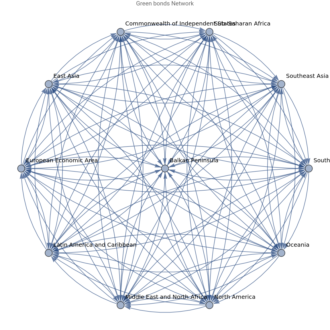
Visualization of the graph model representing the weighted, directed, and aggregate network which represents financial transactions between regions. Edges represent aggregated allocations between regions over the 2006-2017 period.
The simulated region - to - region transfer network as created in Mathematica . Edges represent aggregated allocations between regions over the 2006 - 2017 period .
In[]:=
rb=WeightedAdjacencyGraph[{"Balkan Peninsula","Commonwealth of Independent States","East Asia","European Economic Area","Latin America and Caribbean","Middle East and North Africa","North America","Oceania","South Asia","Southeast Asia","Sub-Saharan Africa"},r11,VertexLabels"Name",PlotLabel"Green bonds Network",ImageSizeLarge,GraphLayout"RadialDrawing",ImagePadding20]
Out[]=
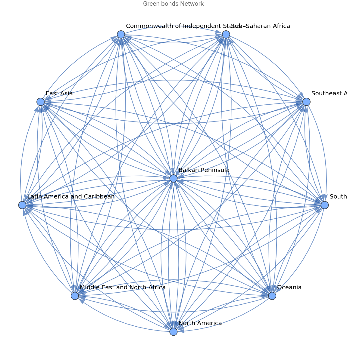
Create a graph by deleting a specific region and all edges connected to this region from graph rb. The output performs a what if scenario analysis: the green bond network, excluding any selected region. The excluded region is selected from a drop-down list at the top left corner of the output cell.
In[]:=
region={"Balkan Peninsula","Commonwealth of Independent States","East Asia","European Economic Area","Latin America and Caribbean","Middle East and North Africa","North America","Oceania","South Asia","Southeast Asia","Sub-Saharan Africa"};
In[]:=
Manipulate[VertexDelete[rb,reg],{{reg,"European Economic Area","Without region:"},region},SaveDefinitions->True]
Out[]=

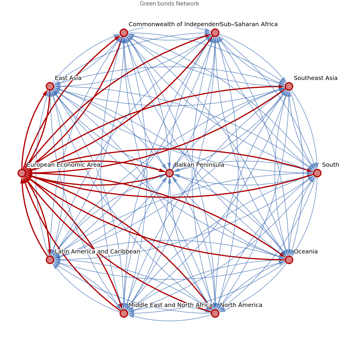
Create a customized graph that highlights the connections of selected nodes (regions). The output presents the connectivity of regions in the global green bond network . Connections are the transactions between regions . The connections of the selected region in the drop - down list are marked in red in the background of the global green bond transfer network.
In[]:=
Manipulate[HighlightGraph[rb,Graph[IncidenceList[rb,reg],VertexLabelsAutomatic,ImageSizeLarge],VertexLabelsAutomatic,VertexLabelStyleBackground->White,GraphHighlightStyle"Thick"],{{reg,"European Economic Area","Connections of region:"},region},SaveDefinitions->True]
Out[]=
Input the weighted adjacency matrices for each allocation year. Author’s Note: The original data used in the paper (Tsilika, 2024) are not used here. These numbers are synthetic and meant for illustrative purposes only.
r2006=;r2007=;r2008=;r2009=;r2010=;r2011=;r2012=;r2013=;r2014=;r2015=;r2016=;r2017=;
Concatenate weighted adjacency matrices for all allocation years.
Program functions weightedout (weightedin) to calculate node strength - out (strength - in) . weightedout (weightedin) takes as argument k the k - th year of the study period . Node strength si sums up the weights of the edges of a given node i .
Create the graph g with all counterparties as nodes and using the weighted adjacency matrix.
The codes present each weighted adjacency matrix, using the TableForm function and highlight the nodes of graph g using HighlightGraph function with the option VertexSize that specifies the size used for nodes (here according to their strength - out). The output constitutes an interactive dashboard for the green bond market. The allocation year is selected from a drop-down list at the top left corner of the output cell. Yearly allocators’ activity is reflected in the weighted adjacency matrix and the green bond allocators’ network. The size of the node is analogous to its strength-out. The bigger the size the more financial flows are transferred from the allocator region to recipient regions.
Load package IGraphM.
The output includes: Up : A heatmap illustrates the Allocators ► Receivers ▼ pattern for allocation proceeds . Down: The region - to - region green bond transfer network with a tooltip option for edge weights . In the green bond allocators’ network (left), node size is proportional to their strength - out . In the green bond receivers’ network (right), node size is proportional to their strength - in . The allocation year is selected from a drop - down list at the top left corner of the output cell .
CITE THIS NOTEBOOK
CITE THIS NOTEBOOK
A Mathematica-based interface for the exploration of inter- and intra-regional financial flows
by Kyriaki Tsilika
Wolfram Community, STAFF PICKS, January 17, 2025
https://community.wolfram.com/groups/-/m/t/3358622
by Kyriaki Tsilika
Wolfram Community, STAFF PICKS, January 17, 2025
https://community.wolfram.com/groups/-/m/t/3358622