Comparing common dimension estimators for hypergraph
by Rauan Kaldybaev
by Rauan Kaldybaev
The Wolfram Model is a theory that models the universe by a discrete hypergraph (a generalization of a graph where an edge can connect multiple vertices). The hypergraph evolves in discrete time steps according to certain rules - laws of physics. One of the key assumptions of the theory is that as time increases, the discrete hypergraph starts to exhibit the properties of continuous space. In particular, the effective dimension of the hypergraph should approach 3. The question of dimension is thus very important in the model. There are many ways we could estimate the dimension of a hypergraph, but the most common are Myrheim-Meyer estimators, Wolfram-Hausdorff estimators, and midpoint scaling estimators. The current computational essay compares the estimators by their speed of convergence and numerical robustness. To make the comparisons, it uses wm1268, wm2224, wm3255 and wm1811 from the Registry of Notable Universes. It appears that the Wolfram-Hausdorff dimension estimator is the best of the three, converging fastest and being the most robust.
In[]:=
Show[wm1811[200]["FinalStatePlot"],ImageSizeLarge]
Out[]=
Getting started
Getting started
Source code for the dimension estimators
Source code for the dimension estimators
The current subsection contains the source code for the dimension estimators. Jonathan Gorard was kind to share the code for Myrheim-Meyer and Wolfram-Hausdorff dimension estimators. The code for midpoint scaling estimator I’ve wrote myself.
Myrheim-Meyer dimension estimator
Myrheim-Meyer dimension estimator
Wolfram-Hausdorff dimension estimator
Wolfram-Hausdorff dimension estimator
Midpoint scaling estimator
Midpoint scaling estimator
Shortcuts
Shortcuts
To compare the three dimension estimators, we can define functions that would take in a WolframModelEvolutionObject and return an estimate for its dimension:
In[]:=
ClearAll[mmDim, whDim, msDim];mmDim[wm_] := MyrheimMeyerDimensionEstimator@wm["CausalGraph"];whDim[wm_] := WolframHausdorffDimensionEstimator[ResourceFunction["HypergraphToGraph"][wm["FinalState"]], "Dimension"];msDim[wm_] := midpointScalingEstimator@wm["CausalGraph"];
Preparing the universes
Preparing the universes
Although most hypergraphs don’t resemble any -dimensional object, some of them actually do have a pretty obvious dimension - for example, some graphs look like long chains of vertices and thus resemble one-dimensional lines. Let us examine wm2224, wm1268, wm3255, and wm1811 from the Registry of Notable Universes. They all appear to have dimension 1 and thus are particularly useful, since the fact that the actual dimension is known makes it easier to validate the output of the dimension estimation algorithms. The following functions allow us to compute the state of each of these universes after steps:
n
n
In[]:=
ClearAll[wm2224, wm1268, wm3255, wm1811];wm2224[n_] := ResourceFunction["WolframModel"][{{{1, 2}, {2, 3}} {{4, 2}, {2, 4}, {4, 3}, {1, 4}}}, {{1, 1}, {1, 1}}, n];wm1268[n_] := ResourceFunction["WolframModel"][{{{1, 1, 2}, {3, 4, 2}} {{4, 4, 2}, {1, 5, 2}, {1, 5, 3}}}, {{1, 1, 1}, {1, 1, 1}}, n];wm3255[n_] := ResourceFunction["WolframModel"][{{{1, 2, 1}, {1, 3, 4}} {{4, 5, 4}, {5, 4, 2}, {3, 2, 5}}}, {{1, 1, 1}, {1, 1, 1}}, n];wm1811[n_] := ResourceFunction["WolframModel"][{{{1, 1, 2}, {1, 3, 4}} {{4, 4, 3}, {2, 5, 3}, {2, 5, 3}}}, {{1, 1, 1}, {1, 1, 1}}, n];
Comparing point estimates
Comparing point estimates
To compare the algorithms for dimension estimation, the most obvious thing to do is to compare the values they output for some selected inputs. This would allow us to make conclusions about the characteristics and speed of convergence of each of the algorithms. Based on the computational experiments below, it can be concluded that the Wolfram-Hausdorff dimension estimator and the midpoint scaling estimator converge faster than Myrheim-Meyer. Although the three algorithms generally agree on what the dimension of a particular object is, in some cases they give drastically different answers because their working principle is very different. A good example is wm2224, which is basically a chain of vertices forming a circle. The Wolfram-Hausdorff estimator looks at the structure of the hypergraph and decides that the universe is one-dimensional. Myrheim-Meyer, however, looks at the structure of the causal graph, which is a tree graph, and thinks that the universe has no definite dimension. In this sense the Wolfram-Hausdorff estimator can be preferable because it operates with more concrete objects. The curvature midpoint estimator also looks at the structure of the causal graph, but miraculously it still manages to give the correct answer 1.
wm1268
wm1268
First, run the dimension estimators on wm1268:
In[]:=
Show[{ListLinePlot[Join@Transpose@Table[Block[{wm=wm1268[n]},{{n,mmDim[wm]},{n,whDim[wm]},{n,msDim[wm]}}],{n,1,40}],PlotLegends{"Myrheim-Meyer","Wolfram-Hausdorff","Midpoint scaling"},AxesLabel{"time","dim"},PlotLabel"wm1268",PlotRangeAll],Plot[1,{n,1,40},PlotStyle{Thin,Dashed,Black}]}]
Out[]=
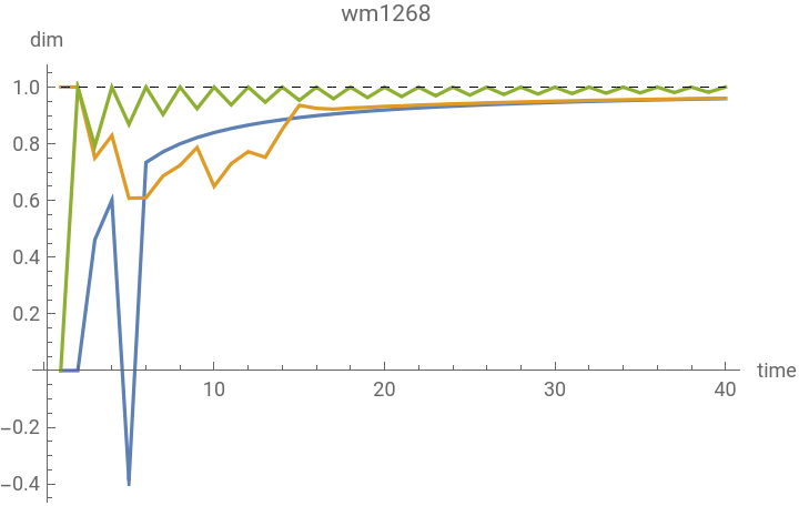


Here, the vertical axis is the estimate for dimension and the horizontal axis is the number of evolution discrete time steps. Although the estimators give crazy results for small , eventually they all three estimators agree that the dimension of the graph is around 1. This makes sense: at the beginning, the graph is small and thus does not exhibit any manifold properties. As time goes by, however, the graph does approach a certain structure. To compare the speed of convergence of the algorithms, plot the difference between the estimates and 1 as a function of time:
n
In[]:=
mmDimErrData1268 = Table[{n, 1 - mmDim[wm1268[n]]}, {n, 25, 205, 20}];whDimErrData1268 = Table[{n, 1 - whDim[wm1268[n]]}, {n, 25, 205, 20}];msDimErrData1268 = Table[{n, 1 - msDim[wm1268[n]]}, {n, 25, 105, 20}];
In[]:=
ListLinePlot[Join[{mmDimErrData1268,whDimErrData1268,msDimErrData1268}],PlotLegends{"Myrheim-Meyer","Wolfram-Hausdorff","Midpoint scaling"},AxesLabel{"time","dim"},PlotLabel"wm1268",PlotRangeAll]
Out[]=
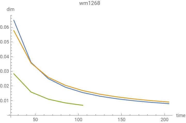
Here, the plot of error for the midpoint scaling estimator stops at 105 because of its slow implementation. It can be seen that while Myrheim-Meyer and Wolfram-Hausdorff estimators converge at approximately the same speed, the midpoint scaling estimator actually seems to be doing significantly better. Also, the error of Myrheim-Meyer and Wolfram-Hausdorff estimators is amazingly accurately modeled by a function:
/n
In[]:=
Block[{model=Normal@LinearModelFit[Join[mmDimErrData1268,whDimErrData1268],1/n,n,IncludeConstantBasisFalse]},Legended[Show[{ListLinePlot[Join[{mmDimErrData1268,whDimErrData1268}],AxesLabel{"time","dim"},PlotLabel"wm1268",PlotRangeAll],Plot[model,{n,Min@mmDimErrData1268[[All,1]],Max@mmDimErrData1268[[All,1]]},PlotStyle{Thick,Dashed,Red},PlotRangeAll]}],LineLegend[{ColorData[97][1],ColorData[97][2],Red},{"Myrheim-Meyer","Wolfram-Hausdorff",Row[{"Model: ",model}]}]]]
Out[]=
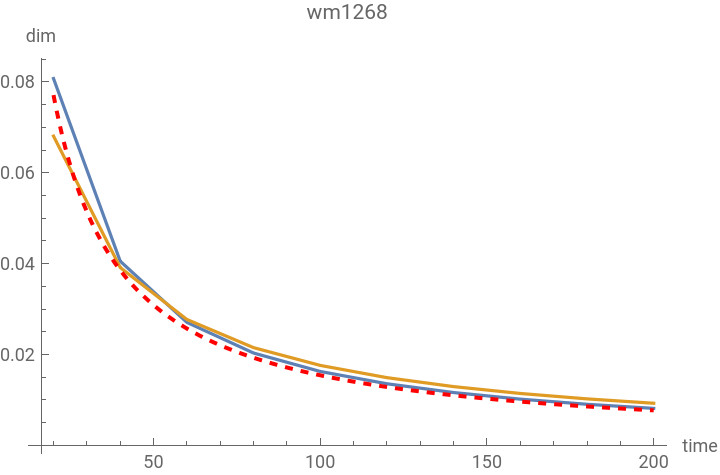


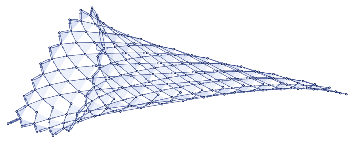
If the trend continues, the error should approach in about 15 000 steps. Considering that the Wolfram Model predicts the Universe to be much much older than that, we can see this as an example of how a discrete graph starts exhibiting manifold properties. This makes sense, as wm1268 basically develops into a tube:
-4
10
wm2224
wm2224
wm3255
wm3255
wm1811
wm1811
Comparing numerical robustness
Comparing numerical robustness
Source code
Source code