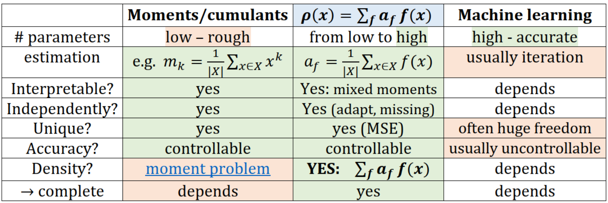
Article Abstract: Machine learning (e.g. artificial neural networks) usually use very large models, often estimated through costly iteration. They lack control of parameters, which are usually non-unique, dependent and difficult to interpret. From the opposite side there is classical statistics using e.g. moments/cumulants which are directly estimated in inexpensive way, unique, well controlled, calculated independently, and have natural interpretations. However, these are usually a few parameter models - offering only a rough description. We will discuss Hierarchical Correlation Reconstruction (HCR) allowing to combine their advantages: use a large number of moment-like parameters, optimized to reconstruct (joint) probability distributions in hierarchical way - first marginal distributions, then pairwise correlation corrections, then triple-wise and so on, also in evolving way for nonstationarity analysis.
While there is a general focus on prediction of values, real data usually only allows to predict (conditional) probability distributions, what is relatively difficult. Standard methods are KDE (kernel density estimation) - rather terrible above 1D, and copulas popular in economics - very low parametric. This article introduces to HCR (hierarchical correlation reconstruction) - a very general family of methods modelling (joint) density as just a linear combination: for orthonormal family e.g. polynomial or Fourier.
ρ(x)(x)
∑
i
a
i
f
i
{}
f
i
Orthonormality allows for inexpensive, independent estimation as just mean over dataset. This way coefficients are close to moments, mixed moments for multiple variables, optimized for direct reconstruction of the estimated density . Using moments makes it great at generalization - further there is 2D example on real data where HCR improves cross-validation log-likelihood evaluation properly describing very subtle dependencies, while KDE turns out worse than trivial model.
Such densities can be also estimated as evolving in time for nonstationary time series, directly predicted for conditional distributions, allow for optimal use for missing data, and many others - discussed in articles ([1],[2],[3],[4],[5],[6],[7],[8],[9],[10],[11],[12],[13]) and briefly below. Here are slides gathering them (recorded talk), some of which were used for this article.
a
i
f
i
a
i
ρ
Such densities can be also estimated as evolving in time for nonstationary time series, directly predicted for conditional distributions, allow for optimal use for missing data, and many others - discussed in articles ([1],[2],[3],[4],[5],[6],[7],[8],[9],[10],[11],[12],[13]) and briefly below. Here are slides gathering them (recorded talk), some of which were used for this article.
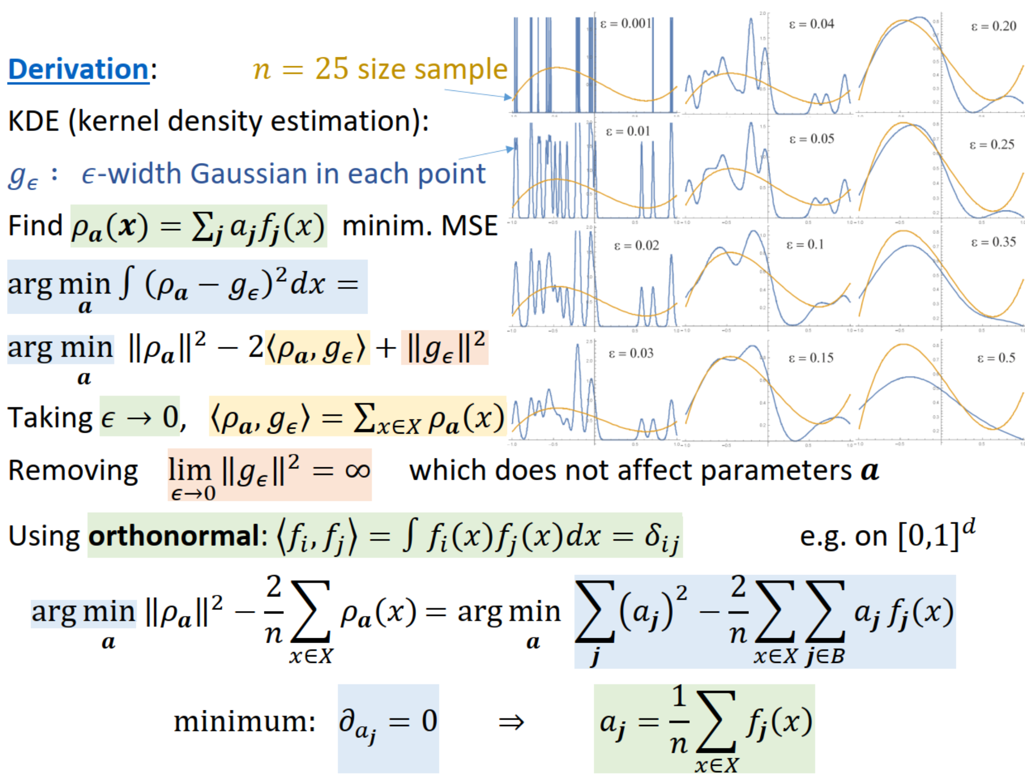
Below is sketch of derivation (details in [1]) of such coefficient estimation as just mean - we smoothen the sample with KDE for kernel radius , and find the coefficients of linear combination minimizing distance (MSE). For orthonormal basis the optimal coefficients can be estimated independently as just averages of functions over the sample.
ϵ0
2
L
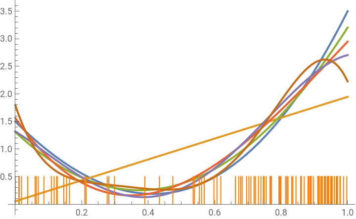
Let us start with 1D case - below one can postulate a density ρ on [0,1] range, there are generated pts random points from this density (marked orange). From these points there is estimated density as a linear combination of orthonormal polynomials (Legendre) by just averaging their value over the sample. The plot shows the real density (blue) and estimated from the generated sample using the written various degree polynomials.
In[]:=
pts=100;mm=5;(*numberofgeneratedpointsandmaximalpolynomialdegree*)ρ=2x^3+6(x-1/2)^2;(*assumeddensityin[0,1]-hastobenonnegativeandintegrateto1*)dt=Interpolation[Table[{Integrate[ρ,{x,0,y}],y},{y,0,1,0.001}]][RandomReal[{0,1},pts]];(*generatesample*)basis=Expand[Table[LegendreP[m,x]*Sqrt[(2m+1)]/.x->2x-1,{m,mm}]];(*orthonormalbasis*)a=Map[Mean,basis/.x->dt];(*ESTIMATECOEFFICIENTSinbasis*)pd=Graphics[{Orange,Table[Line[{{v,0},{v,0.5}}],{v,dt}]}];(*plotsample*)rhos=Prepend[Table[1+Total[(basis*a)[[1;;m]]],{m,mm}],ρ];(*estimateddensities*)Show[Plot[rhos,{x,0,1},PlotLegends->Prepend[Range[mm],"real ρ"]],pd]
Out[]=


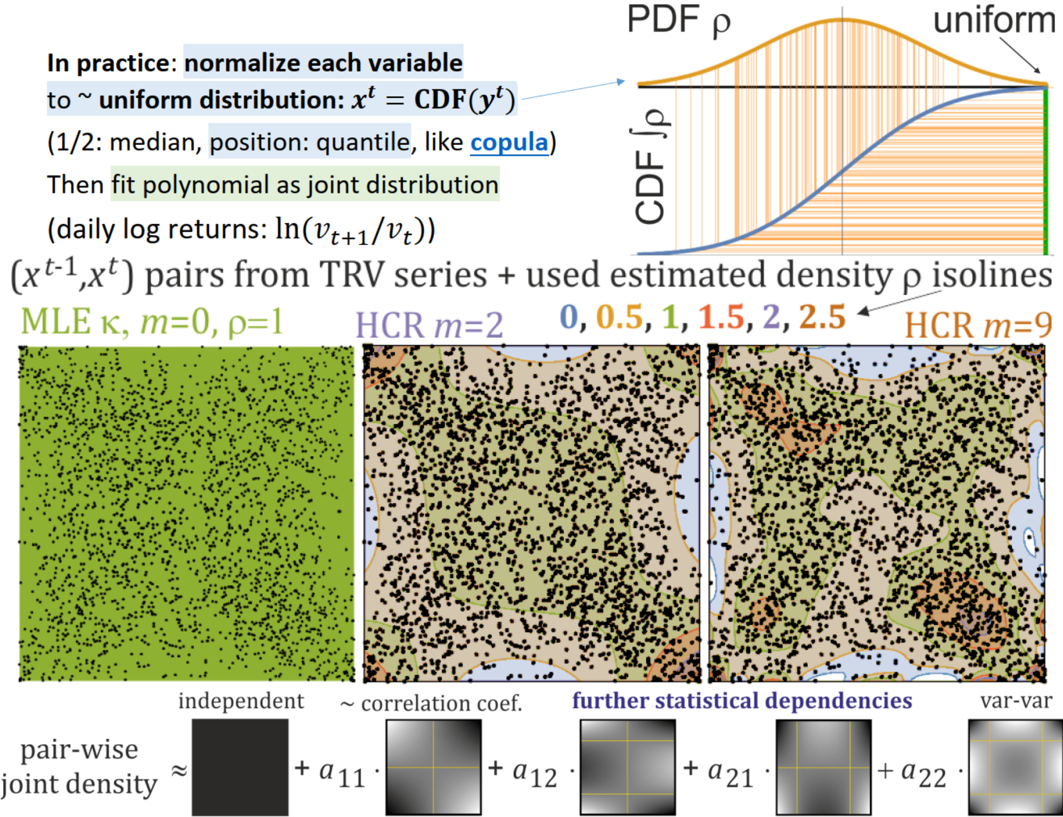
For multiple variables we can e.g. use product basis like (x,y)(x)(y) as orthonormal. This way coefficients describe mixed moments between two variables. While not necessary, it is very practical to first normalize the variables to nearly uniform on [0,1] like in copulas - to approximately quantiles of the corresponding values. It is done by estimating CDF (cumulative distribution function) for the variable and using as the final variable. This estimation can be done using some parametric distribution like Gaussian with estimated parameters. If none fits to the given data, we can also always use empirical distribution function - sort the values and assign to positions in such ordering rescaled to [0,1].
f
ij
f
i
f
j
a
ij
xCDF(y)
We can also use more sophisticated normalization, e.g. with time dependent CDF to include nonstationarity, for example with ARMA-ARCH popular models, or some based on exponential moving average like proposed and usually superior: adaptive exponential power distribution or adaptive Student’s t-distribution.For two variables normalized to nearly uniform distribution on [0,1], if independent their joint density would be just on . Usually 1 corresponding to normalization, this way coefficients describe marginal distribution of the first variable (e.g. corrections to normalization), of the second variable. Then describes dependence of expected values, and is usually close to the Pearson correlation coefficient. Then describes statistical dependency between i-th moment of the first variable and j-th moment of the second variable, e.g. for common variance-variance dependence as so called homoscedasticity.
ρ≈1
2
[0,1]
f
0
a
i0
a
0j
a
11
a
ij
a
22
Analogously for more variables, e.g. (x,y,z)(x)(y)(z) product basis adds triple-wise dependencies. As 1, zero index means there is no dependence of given variable, allowing literally for hierarchical correlation reconstruction (HCR) as in the name - start with the details of marginal distributions using coefficients having single nonzero index, then add pairwise dependencies with coefficients having two nonzero indexes, and so on. Here are such bases in for d = 1, 2, 3 variables:
f
ijk
f
i
f
j
f
k
f
0
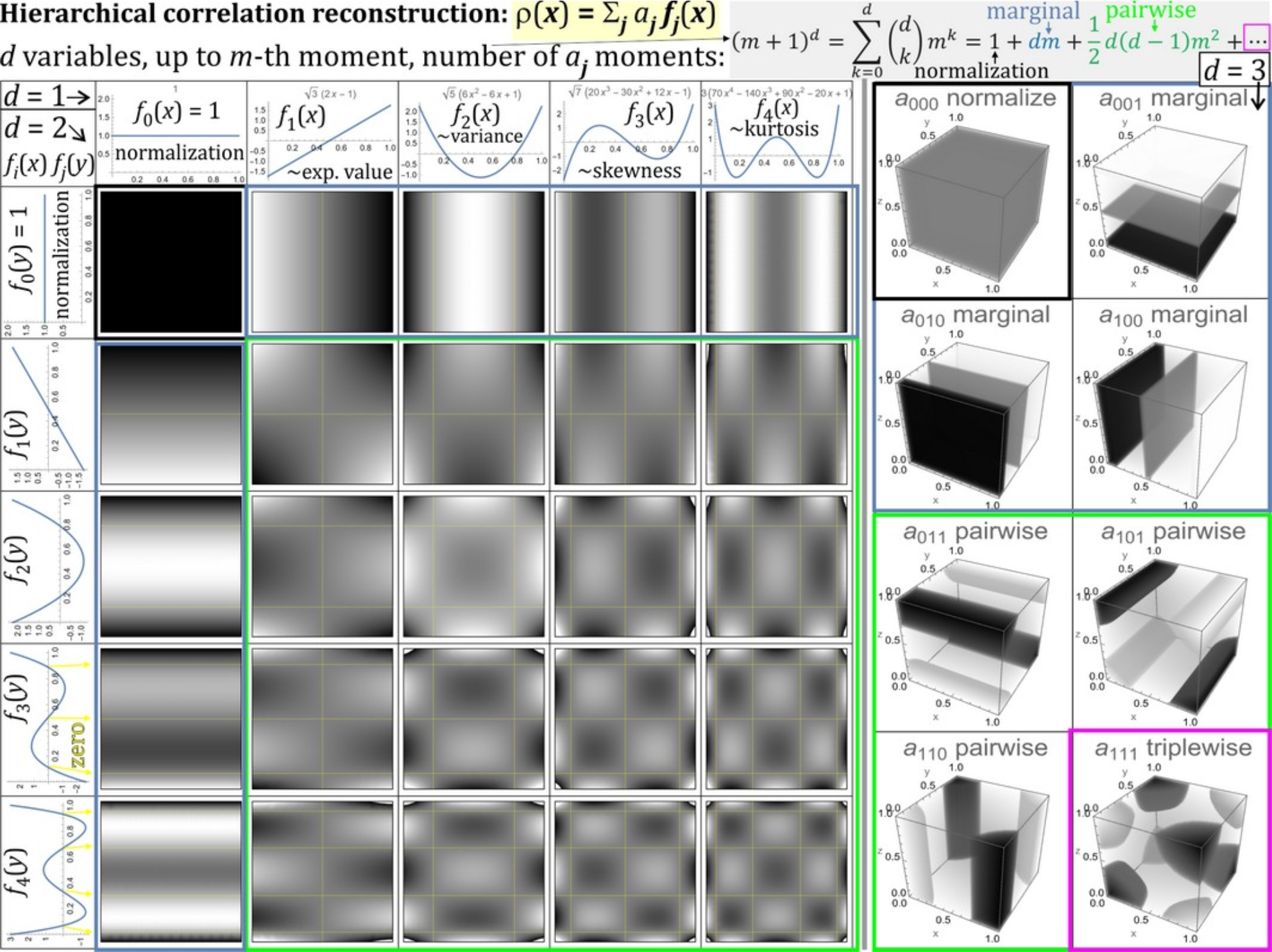
Obviously the size of such basis grows exponentially with the number of variables - requiring some restrictions for the set of used coefficient, or mentioned later direct prediction of conditional distribution. Such hierarchical decomposition is also perfect for missing data situations - if only a subset of variables is available, we still can use such incomplete vector to improve estimation of all dependencies it contains.
Let us now estimate joint distribution of some real economical data: log-returns normalized with popular Student's t-distribution. There are calculated pairs of succeeding normalized log-returns (dots), for which there is estimated density (contours) using complete pairwise basis up to degree m.
Let us now estimate joint distribution of some real economical data: log-returns normalized with popular Student's t-distribution. There are calculated pairs of succeeding normalized log-returns (dots), for which there is estimated density (contours) using complete pairwise basis up to degree m.
In[]:=
m=6;(*msizebasisformarginaldistribtutions+forpairwisejointdistrbituion*)dat=FinancialData["DJI","Price",{2000,1,1}][[2,1,1]];(*importtimeseries*)lr=Log[dat[[2;;-1]]/dat[[1;;-2]]];(*calculatelog-returns*)ndat=CDF[EstimatedDistribution[lr,StudentTDistribution[μ,σ,ν]],lr];(*normalize*)pairs=Transpose[{ndat[[1;;-2]],ndat[[2;;-1]]}];(*pairsofsucceedingvalues*)basis=Expand[Table[LegendreP[i,x]*Sqrt[(2i+1)]/.x->2x-1,{i,0,m}]];(*basis*)pval=Prepend[basis[[2;;-1]]/.x->Transpose[pairs],Table[1.,2,Length[pairs]]];a=Table[Mean[pval[[i,1]]*pval[[j,2]]],{i,m+1},{j,m+1}];(*estimatecoefficients*)rho=basis.a.(basis/.x->y);(*estimateddensity,plotdensityandpoints:*)Show[ContourPlot[rho,{x,0,1},{y,0,1},PlotLegends->Automatic],Graphics[Point[pairs]]]
2
m
the same using KDE - only negative log-likelihood: worse than just rho=1
Below is analogous basic density estimation for triples of succeeding normalized log-returns.
Below is Parametric Density Estimation Using Polynomials and Fourier Series interactive demonstration from Wolfram Demonstration Project, allowing to manually insert points also for clustering application by using opposite weights, for basis as polynomials or Fourier:
Let us now briefly discuss some basic further modifications/extensions. One very practical is direct prediction of conditional probability distributions ([5],[6],[9],[10]). While we could predict it from some model of joint distribution like above, especially for a large number of variables it leads to numerical issues - direct prediction allows for practical estimation of conditional distributions also from very large numbers of variables of various types (continuous, discrete, mixed). Specifically, we represent conditional probability distribution of the predicted variable Y as a linear combination like previously (can be multivariate), and directly predict its coefficients from features of the remaining variables - e.g. using linear regression, but could be also more sophisticated like neural networks: replacing prediction of value with prediction of a few moments, further used to reconstruct conditional probability distribution.
We can also perform multi-feature correlation analysis: looking at two time series, or one for various time differences (lag below), they usually have some complex joint distributions. Usually there is just calculated correlation, while with HCR we can calculate multiple mixed moments, and find dominant contributions to joint distributions e.g. with PCA - getting multiple dominant statistical dependencies, and analyze their time evolution e.g. to search for hidden subtle periodic processes e.g. of blazars below [7], for better understanding of contagion between financial markets [8], vibration analysis e.g. bearing diagnosis [12], or analyze multi-feature Granger causality e.g. for EEG data [11].
A promising directions is application of HCR for artificial neurons ([2], [13]) with separate notebook. While standard artificial neural networks are optimized for unidirectional propagation, in biological neurons action potential travels in both directions (e.g. https://journals.aps.org/pre/abstract/10.1103/PhysRevE.92.032707 ), hence evolutionariliy they should be optimized for for such mulitidirectional operation, what might be essential especially for learning - currently not well understood. HCR offer inexpensive joint distribution neuron - allowing for propagation in any direction as conditional distributions. Beside standard backpropagation, such structure allows for additional training approaches which might be exploited by biological neurons - e.g. with direct parameter estimation, feature extraction, or tensor decompositon.
Here are 2 and 3 variable examples of such propagation in any direction as conditional density, or its expected values. The code is available in https://community.wolfram.com/groups/-/m/t/3241700
Finally, here is a summary of adventures of prediction of probability distribution e.g. using HCR:
References
References
[2] J. Duda, Hierarchical correlation reconstruction with missing data, for example for biology-inspired neuron, arXiv:1804.06218 (2018)
[3] J. Duda, Exploiting statistical dependencies of time series with hierarchical correlation reconstruction, arXiv:1807.04119 (2018)
[4] J. Duda, M. Snarska, Modeling joint probability distribution of yield curve parameters, arXiv:1807.11743 (2018)
[5] J. Duda, A. Szulc, Credibility evaluation of income data with hierarchical correlation reconstruction, arXiv:1812.08040 (2018), International Conference on Applied Economics (2020)
[6] J. Duda, R. Syrek, H. Gurgul, Modelling bid-ask spread conditional distributions using hierarchical correlation reconstruction, arXiv:1911.02361(2019), Statistics in Transition vol 21 no 4 (2020)
[7] J. Duda, G. Bhatta, Log-stable probability density functions, non-stationarity evaluation, and multi-feature autocorrelation analysis of the γ-ray light curves of blazars, arXiv:2005.14040 (2020), Monthly Notices of the Royal Astronomical Society Main Journal (2021)
[8] J. Duda, H Gurgul, R. Syrek, Multi-feature evaluation of financial contagion, Central European Journal of Operations Research (2021)
[9] J. Duda, G. Bhatta, Predicting conditional probability distributions of redshifts of Active Galactic Nuclei using Hierarchical Correlation Reconstruction, arXiv:2206.06194 (2022), Monthly Notices of the Royal Astronomical Society Main Journal (2024)
[10] J. Duda, S.Podlewska, Low cost prediction of probability distributions of molecular properties for early virtual screening, arXiv:2207.11174, Molecular Diversity (2022)
[11] J. Duda, Time delay multi-feature correlation analysis to extract subtle dependencies from EEG signals, arXiv:2305.09478 (2023)
[12] J. Duda, J. Leśkow, P. Pawlik, W. Cioch, CMAFI — Copula-based Multifeature Autocorrelation Fault Identification of rolling bearing, Mechanical Systems and Signal Processing (2024)
[13] J. Duda, Biology-inspired joint distribution neurons based on Hierarchical Correlation Reconstruction allowing for multidirectional neural networks, arXiv:2405.05097 (2024)
CITE THIS NOTEBOOK
CITE THIS NOTEBOOK
Hierarchical correlation reconstruction: between statistics and machine learning
by Jarek Duda
Wolfram Community, STAFF PICKS, September 21, 2023
https://community.wolfram.com/groups/-/m/t/3017754
by Jarek Duda
Wolfram Community, STAFF PICKS, September 21, 2023
https://community.wolfram.com/groups/-/m/t/3017754