Introduction
Introduction
The wave equation is a linear second order partial differential equation that describes the propagation of waves . In its two - dimensional form, it contains a time variable , two spatial variables and a function of these variables, u, that describes the displacement of a medium through which waves are propagating over time . That the wave equation is linear implies that its solution can consist of the sum of any number of solutions . This is observed in nature as the superposition principle wherein waves add constructively and destructively when occupying the same space . Using Fourier series to model wave behavior in a two - dimensional membrane is, then, appropriate in that the sums of sines and cosines can be used to approximate the total displacement of the membrane over its surface area . The solution of the two - dimensional wave equation for a rectangular membrane that is fixed at its boundaries can be found through separation of variables and the application of both boundary conditions and initial conditions, and expressed as a double Fourier series . From the solution, the behavior of the membrane as waves propagate through it can then be explored by introducing an initial displacement and/or initial velocity in its surface .
(t)
(x,y)
2D Wave Equation in Cartesian Coordinates
2D Wave Equation in Cartesian Coordinates
The wave equation for a two - dimensional rectangular membrane with boundary and initial conditions is expressed as
u
tt
2
c
u
xx
L
x
L
y
u(0,y,t)u(,y,t)0, t≥0
L
x
u(x,0,t)u(x,,t)0, t≥0
L
y
u(x,y,0)f(x,y), (x,y)g(x)0≤x≤, 0≤y≤
u
t
L
x
L
y
where u(x, y, 0) and u t (x, y, 0) are the initial displacement and velocity of a membrane fixed at its edges. c is the propagation velocity of the wave, or the square root of the tension per length of the membrane dividedby its surface density while and are the lengths of the membrane in the and directions,respectively.This model assumes no external forces or damping.
T
ρ
L
x
L
y
x
y
Solving the Wave Equation
Solving the Wave Equation
We set and , , for the above problem.
f(x,y)x*y(1-x)(1-y)
g(x)0
c4
L1
Using the method separation of variables we will try to find the general solution of the problem .
Let assume a solution in the form
u(x,y,t)X(x)Y(y)T(t)
so that substitution into the partial differential equation (PDE) results in
′′
T
2
c
′′
X
′′
Y
It follows that when rearranged,
′′
T
2
c
′′
X
X(x)
′′
Y
Y(y)
the left side is dependent only upon while the right is dependent upon and . If both sides are equal to one another with any or they must also be equal to some constant. We choose , so that the independent variables, and can ultimately be expressed in terms of sines and cosines. With
t
x
y
t,x
y,
-
2
λ
T,X
Y
′′
T
2
c
′′
X
X(x)
′′
Y
Y(y)
2
λ
the terms form the second order differential constant coefficient homogeneous equation
T
T(t)cos(cλt)+sin(cλt)(1)
k
1
k
2
From Equation , the and terms can also be set to constants such that
(1)
X
Y
′′
X
X(x)
2
λ
′′
Y
Y(y)
2
λ
′′
Y
Y(y)
2
ν
′′
Y
Y(x)
2
λ
′′
X
X(y)
2
λ
′′
X
X(y)
2
μ
Solving for and in a similar manner as was applied to gives
X
Y
T
X(x)cos(νx)+sin(νx)
a
1
a
2
Y(x)cos(μx)+sin(μx)
b
1
b
2
Substituting the solutions for and Y into results in
T,X
u(x,y,t)T(t)X(x)Y(y)
u(x,y,t)[cos(cλt)+sin(cλt)]·[cos(νx)+sin(νx)]·[cos(μx)+sin(μx)]
k
1
k
2
a
1
a
2
b
1
b
2
The boundary conditions (BC) which must be satisfied are then applied to and to find and .
X(x)
Y(y)
ν
μ
Beginning with the boundaries in the dimension at and where , we have
X
x0
x
L
x
u(0,y,t)u(,y,t)0
L
x
X(0)cos(0)+sin(0)0
a
1
a
2
a
1
X(x)sin(νx)
a
2
X()sin(ν0)
L
x
a
2
L
x
If is chosen to equal , then we arrive at a trivial solution with Because a trivial solution is not desired, when the argument of the sine function is some integer multiple of (namely, ) so that . A similar result is found in applying the dimension boundary conditions to where 0 and . Combining Equations and leads to
a
2
0
u(x,y,t)0.
X()0
L
x
π
νnπ
L
x
ν
nπ
L
x
Y
Y(y),
b
1
μ
mπ
L
y
(1),(2)
(3)
′′
X
X(x)
′′
Y
Y(y)
2
ν
2
μ
2
λ
λ+
2
ν
2
μ
Because all three variables are functions of n and m, they can now be expressed as
ν
n
nπ
L
x
μ
m
mπ
L
y
λ
nm
2
v
n
2
μ
m
Then using the initial conditions for the case and (the initial velocity equals to zero)
f(x,y)x*y(1-x)(1-y)
g(x,y)0
u(x,y,t)=sinsincos+t
∞
∑
n=1
∞
∑
m=1
a
nm
nπx
L
mπy
L
cπ
L
2
n
2
m
a
nm
4
2
L
L
∫
0
L
∫
0
nπx
L
mπy
L
Running the following code on Mathematica will produce the solution of the problem
In[]:=
Clear["Global`*"]c=4;L=1;
(*Definitionoffunctionsf(x,y)andg(x,y)*)f[x_,y_]:=x*y(1-x)*(1-y)g[x_,y_]:=0μ[n_]=(n*π)^2;κ[m_]=(m*π)^2;λ[n_,m_]=μ[n]+κ[m];ω[n_,m_]=c*Sqrt[λ[n,m]]//SimplifyU[n_,m_]=Sin[(n*π*x)/L]*Sin[(m*π*y)/L]
Out[]=
4+π
2
m
2
n
Out[]=
Sin[nπx]Sin[mπy]
(*ComputationoftheFouriercoefficients*)A[n_,m_]=4/L^2f[x,y]*U[n,m]xy
L
∫
0
L
∫
0
Out[]=
4(-2+2Cos[mπ]+mπSin[mπ])(-2+2Cos[nπ]+nπSin[nπ])
3
m
3
n
6
π
In[]:=
B[n_,m_]=4/(L^2*ω[n,m])g[x,y]*U[n,m]xy
L
∫
0
L
∫
0
Out[]=
0
The general solution of our problem
The general solution of our problem
u1[x,y,t]=(A[n,m]*Cos[ω[n,m]*t]+B[n,m]*Sin[ω[n,m]*t])*Sin[(n*π*x)/L]*Sin[(m*π*y)/L]
Out[]=
1
3
m
3
n
6
π
2
m
2
n
u[x_,y_,t_,l_,k_]:=
l
∑
n=1
k
∑
m=1
16(-1+)(-1+)Cos+πtSinSin
m
(-1)
n
(-1)
2
m
2
n
nπx
L
mπy
L
3
m
3
n
6
π
We calculate the partial sum (k,l)=(1,1),(2,1),(2,2),(3,3)
We calculate the partial sum (k,l)=(1,1),(2,1),(2,2),(3,3)
u[x,y,t,1,1]//TraditionalFormu[x,y,t,1,2]//TraditionalFormu[x,y,t,2,2]//TraditionalFormu[x,y,t,3,3]//TraditionalForm
Out[]//TraditionalForm=
64cos(
2
πt)sin(πx)sin(πy)6
π
Out[]//TraditionalForm=
64cos(
2
πt)sin(πx)sin(πy)6
π
Out[]//TraditionalForm=
64cos(
2
πt)sin(πx)sin(πy)6
π
Out[]//TraditionalForm=
64cos(
2
πt)sin(πx)sin(πy)6
π
64cos(
10
πt)sin(3πx)sin(πy)27
6
π
64cos(
10
πt)sin(πx)sin(3πy)27
6
π
64cos(3
2
πt)sin(3πx)sin(3πy)729
6
π
We plot snapshots for the last case
We plot snapshots for the last case
In[]:=
graphs=Table[ParametricPlot3D[{x,y,u[x,y,t,3,3]},{x,0,2},{y,0,3},Axes->False,Boxed->False,BoxRatios->{1,1,1},ImageSize->600,BoundaryStyle->Directive[Red,Thick],ColorFunction->"MintColors",PlotRange->All],{t,0,2,1/4}];p1=Partition[graphs,3];Show[GraphicsGrid[p1]]
Out[]=
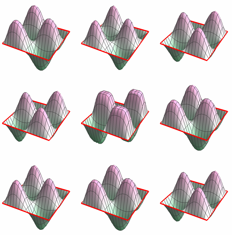
We create a three - dimensional graph
We create a three - dimensional graph
2D Wave Equation in Polar Coordinates
2D Wave Equation in Polar Coordinates
Now we will try to solve another problem with different initial condition
Using the method separation of variables we will try to find the general solution of the problem.
So the general solution of the boundary value problem is the following
Running the following code on Mathematica will produce the solution of the problem
We calculate the first ten terms and the coefficients
We calculate the first ten terms and the coefficients
We plot some snapshots of the solution
We plot some snapshots of the solution
We create a three - dimensional graph
We create a three - dimensional graph
Helmholtz problem in circular disk
Helmholtz problem in circular disk
The following expression
Now we create the 3D graphics
Solving Helmholtz Equation in 2D for Circular Disk with DEigensystem, NDEigensystem
Solving Helmholtz Equation in 2D for Circular Disk with DEigensystem, NDEigensystem
Compute the first 4 eigenfunctions for a circular membrane with the edges clamped:
◼
DEigensystem
◼
NDEigensystem
Nonlinear Schrödinger equation
Nonlinear Schrödinger equation
Numerical Solution
Numerical Solution
3D visualization
3D visualization
Problem 2
Problem 2
CITE THIS NOTEBOOK
CITE THIS NOTEBOOK
A lecture on the wave equation in two dimensions
by Athanasios Paraskevopoulos
Wolfram Community, STAFF PICKS, May 28 2023
https://community.wolfram.com/groups/-/m/t/2926708
by Athanasios Paraskevopoulos
Wolfram Community, STAFF PICKS, May 28 2023
https://community.wolfram.com/groups/-/m/t/2926708