Introduction
Introduction
What could be better for a grand mathematical cheers, than the recent news that a very nice solution has been found to the “ein stein” problem? This famous problem asks for a non-periodic tiling of the plane by a single geometric shape. More precisely, we allow copies of the shape to rotate, translate, and reflect through the plane. Using the many similar pieces, we then attempt to build larger and larger contiguous patches, “topological disks” without overlaps or holes. If arbitrarily large topological disks can always be arranged, and if these patches never conform to symmetry expectations satisfied by the unit cells of a periodic tiling, then the problem is solved. That is the claim of a preprint posted earlier this week. The purpose of this memo is not to re-prove the claim, but merely to take the first steps in that direction by providing explicit construction of Hat Tiling patches by a Local Derivation from the HPTF substitution tiling.
The hat tile is a “4-polykite”, meaning that it’s made of four kites, which are really 1/3 dissections of a hexagon (as is shown in Fig. 1.1 of the original paper). Thus edge lengths measure either 1, 2, or while angles between edges measure in even multiples of π/6 = 30 Degrees. The shape of the tile can be found by taking a walk around its edges:
3
,In[]:=
TileEdgeList[1][dir_:0,ref_:False,pt_:0]:=Module[{res},res={e[Sqrt[3],dir-1],e[Sqrt[3],dir+1],e[1,dir+4],e[1,dir+6],e[Sqrt[3],dir+3],e[Sqrt[3],dir+5],e[1,dir+8],e[1,dir+6],e[Sqrt[3],dir+9],e[Sqrt[3],dir+7],e[1,dir+10],e[2,dir+12],e[1,dir+14]};res=RotateLeft[res,pt];res=If[TrueQ[ref],ReplaceAll[RotateRight[Reverse[res],0],e[len_,x_Integer]:>e[len,Mod[-x,12]]],ReplaceAll[res,x_Integer:>Mod[x,12]]];res]
In[]:=
TilePolygon[Tile[1][or_,dir_,ref_:False,pt_:0]]:=With[{vecs=ReplaceAll[TileEdgeList[1][dir,ref,pt],e[len_,x_]:>Times[len,ReIm[Exp[IPi/6x]]]]},Polygon[FoldList[Plus,or,vecs]]]
In[]:=
Graphics[{LightGray,EdgeForm[Black],TilePolygon[Tile[1][{0,0},0,#]],Red,PointSize[Large],Point[{0,0}]}]&/@{True,False}
Out[]=
,
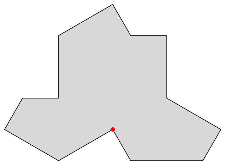
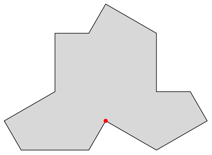
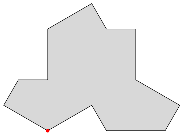
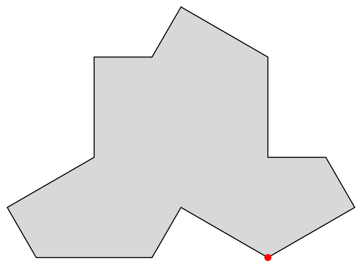
In addition to allowing for reflections, the data model also allows us to shift the origin around the edge of the tile:
In[]:=
With[{shift=1},Graphics[{LightGray,EdgeForm[Black],TilePolygon[Tile[1][{0,0},0,#,shift]],Red,PointSize[Large],Point[{0,0}]}]&/@{True,False}]
Out[]=
,
And we can also rotate the tile:
In[]:=
With[{angle=1},Graphics[{LightGray,EdgeForm[Black],TilePolygon[Tile[1][{0,0},angle,#,1]],Red,PointSize[Large],Point[{0,0}]}]&/@{True,False}]
Out[]=
,
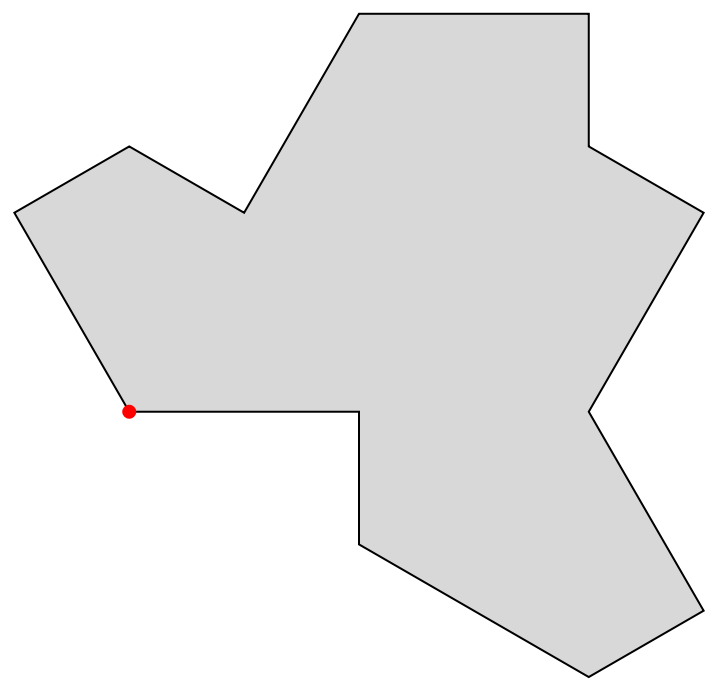
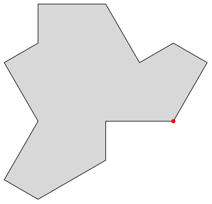
This flexibility will help us later when we need to inset these tiles to another tiling by matching vertex locations.
Assuming we all already know about the Penrose tiling (and maybe a few other inflation tilings such as Trilobite and Crab, and / or the Socolar-Taylor monotile), we could suppose that an inflation rule exists mapping one hat into a larger cluster of hats, while preserving the combinatorics implied by edge shape. This appears not to be true if we allow only one rule, but could likely be done by allowing multiple rules (for example, as done here). We can look for such rules later, but for now we are just going to follow closely what the authors have already done.
The HPTF tiles
The HPTF tiles
In Fig. 2.8 of the original paper, the authors give a substitution system, which looks like most of what we’ve seen in the past except for one caveat. Over levels of the substitution hierarchy, the edge lengths change, only obtaining a fixed point in the infinite limit. In this limit, the HTPF tiles can be thought of as having fractal edges. We can approximate such a limit by again writing the tiles as walks around edges, and then applying substitution rules directly to the edges themselves. Using the notation of Fig. 4.1, the tile edge lists can be written out as follows:
In[]:=
vecReps={A[_][x_]:>6ReIm[Exp[IPi/3x]],B[_][x_]:>6ReIm[Exp[IPi/3x]],F[_][x_]:>2ReIm[Exp[IPi/3x]],X[_][x_]:>2ReIm[Exp[IPi/3x]],L[_][x_]:>2ReIm[Exp[IPi/3x]]};
In[]:=
TileEdgeList["H"][ind_]:={X[1][ind+0],B[0][ind+1],X[0][ind+1],X[1][ind+2],B[0][ind+3],X[0][ind+3],X[1][ind+4],A[1][ind+5],X[0][ind+5]};
In[]:=
TileEdgeList["T"][ind_]:={A[0][ind+0],A[0][ind+2],B[1][ind+4]};
In[]:=
TileEdgeList["P"][ind_]:={X[1][ind+0],A[0][ind+0],L[0][ind+2],X[0][ind+2],X[1][ind+3],B[1][ind+3],L[0][ind+5],X[0][ind+5]};
In[]:=
TileEdgeList["F"][ind_]:={X[1][ind+0],L[0][ind+0],X[0][ind+0],F[1][ind+1],F[0][ind+2],X[1][ind+3],B[1][ind+3],L[0][ind+5],X[0][ind+5]};
These are depicted as follows:
In[]:=
Show[MapThread[Graphics[With[{vecs=ReplaceAll[Flatten[TileEdgeList[#][0]],vecReps]},{Text[Style[#1,Gray,Bold,12],{#2+2,-2}],LightGray,EdgeForm[Black],Polygon[FoldList[Plus,{#2,0},vecs]],Red,PointSize[Large],Point[{#2,0}]}]]&,{{"H","T","P","F"},{0,6,15,26}}]]
Out[]=
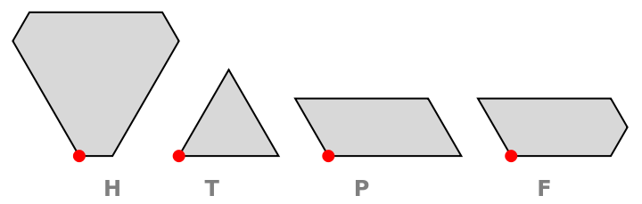
The data model for the HTPF tiles is not quite as flexible, because later we will need canonical forms to translate the replacement rules from Figures 5.15, 5.16, 5.17, 5.18 into code. To start this process, we note that the letters and numbers of our edge representation correspond to colors and symbols in the Figures. From the four figures, we can read off replacement rules for the edges themselves:
In[]:=
edgeReps={A[0][ind_]:>{B[0][ind],X[0][ind],X[1][ind+1]},A[1][ind_]:>{X[0][ind+1],X[1][ind],B[1][ind]},B[0][ind_]:>{X[0][ind+1],X[1][ind],A[0][ind]},B[1][ind_]:>{A[1][ind],X[0][ind],X[1][ind+1]},F[0][ind_]:>{X[1][ind],L[0][ind],X[0][ind],F[1][ind+1]},F[1][ind_]:>{F[0][ind+1],X[1][ind],L[0][ind],X[0][ind]},L[0][ind_]:>{L[0][ind-1]},X[0][ind_]:>{X[0][ind-1],X[1][ind],L[0][ind],X[0][ind],F[1][ind+1]},X[1][ind_]:>{F[0][ind+1],X[1][ind],L[0][ind],X[0][ind],X[1][ind-1]}};
In[]:=
Show[MapThread[Graphics[With[{vecs=ReplaceAll[Flatten[Nest[#/.edgeReps&,TileEdgeList[#][0],4]],vecReps]},{Text[Style[#1,Gray,Bold,12],{#2+2,-100}],LightGray,EdgeForm[Black],Polygon[FoldList[Plus,{#2,0},vecs]],Red,PointSize[Large],Point[{#2,0}]}]]&,{{"H","T","P","F"},{0,450,800,1350}}]]
It’s not ideal that the substitution rule is growing dendrites, but also does not seem to indicate that a mistake has been made. Cutting out the dendrites would be a good idea, for example, if we wanted to represent the edge walk as a pair of integer sequences (vector angle, vector length). But doing so would require splitting some of the edge symbols. We don’t need to do this now, because the existence of dendrites doesn’t interfere with the main thing we need the edge replacement rules: path tracking.
In the subsequent data model for H,T, P, and F tiles, each tile has a local origin and a direction. The local origin gets hooked into the whole tiling by specifying it’s particular value as a summation over other edges in the tiling. This is a neat trick, which allows us to circumvent all the difficulties associated with the substitution system’s running inflation factor. Again, reading the inflation rules off the four figures in Section 5, we find that:
For data of this sort, we need to expand upon our earlier depiction function:
With a little re-scaling, the substitution rules can be depicted as:
As long as we’ve already edited out all the mistakes in our code tables (there were a few, trust me about that), we now have just about everything we need to iterate the replacement rules and obtain ever-larger parts of the substitution tiling.
Putting it all together
Putting it all together
One last thing we need for our data model is a computable form of the original paper’s Figure 4.1. It is now given as:
Unlike the substitution growth rule, the projection from HTPF into hats doesn’t change the size of a patch of the tiling, as we can see here:
With all these tools, the way forward is clear: Iterate the substitution rules, and project final results into hat tiles as necessary. To do so, we introduce a simple inflation iterator:
A basic depiction of the HTPF tiling can be obtained as follows:
And the projection into hats is not much more difficult:
Here, we’ve colored the patch with it’s parity pattern. Of course, we can get more creative with coloring. The following code produces the headliner image at the top of this post:
Now we can realize it’s really not that difficult to generate patches of the tiling, and we can move on to doing some art projects or even to more analysis and characterizing substructure. There’s bound to be more interesting discoveries soon, and I’m looking forward to see what turns out. Congratulations again to the authors on making such an interesting and unexpected discovery!