In our laboratory we are engaged in numerical modeling of processes in quantum dots, using Wolfram Mathematica. In particular, we study optical and light phenomena to quantum dots, such as: interband absorption, photoluminescence, intraband absorption, nonlinear absorption, harmonic generations in quantum dots and much more. In this paper, we will show how to calculate impurity states and plots electrons density in a different quantum dots.
Introduction
Introduction
Impurity states in quantum dots are a significant area of study in modern nanophysics and quantum mechanics. Quantum dots, which are nanoparticles capable of confining and controlling electrons due to their properties associated with particle motion restrictions, exhibit impurity states when foreign atoms or ions are introduced into their structure. These impurities alter the energy levels and quantum properties of the material.
These states play a crucial role in developing new technologies, such as quantum computing, optoelectronics, and photonics. Impurities can enhance quantum dot characteristics, for instance, their ability to absorb light, increase carrier lifetimes, and enable more precise control of spin states.
Such research is particularly relevant for creating quantum computers and sensors, where controlling impurity states can significantly impact device efficiency and reliability. This field promises to lay the groundwork for future innovations, where quantum dots could transform conventional approaches to information processing and light interaction.
Out[]=
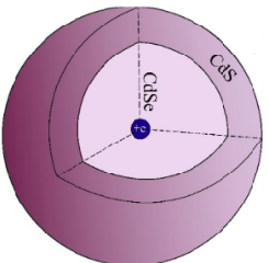
Fig. 1. Impurity in center of Shperical CdS quantum dot
Quantum Dot model
Quantum Dot model
The geometry of semiconductor quantum dots (QDs) plays a crucial role in their optical and electronic properties. Different shapes of QDs allow them to demonstrate unique characteristics that can be utilized in various applications. Here are some of the main geometries of semiconductor QDs:
Let’s start by constructing a top view of a spherical quantum dot:
In[]:=
ClearAll[sphere];sphere[a_] := Region @ ImplicitRegion[ + <= , {x, y}]
2
x
2
y
2
a
Next, we introduce the physical constants and converters that are necessary for calculations
In[]:=
e = 1.602* (* Electron charge in Coulomb*);ϵ0 = 8.854* (* Vacuum permittivity *);ϵ = 15.5 (* Dielectrin constant *);ev = 1.602* (* Converter Joule to Electron Volts *);mev = *ev (* Converter Electron Volts to mili Electron Volts *);nm = (* Converter meters to nanometers *);ℏ = 1.05456* (* reduced Plank cosntant *);m0 = 9.109* (* electron mass *);μ = 0.157*m0 (* electron effective mass *);
-19
10
-12
10
-19
10
-3
10
-9
10
-34
10
-31
10
Based on many works, our task is reduced to solving the following Schrödinger equation
Out[]=

where is reduced Plank cosntant, in electron effective mass in qunatum dot, ψ is electron wavefunction, ϵ is dielectric constant of qunatum dot material, is Vacuum permittivity, is electron charge, ()is electron and impurity coordinates, is the system energy.
m
e
ϵ
0
e
x
e(i)
y
e(i)
E
To begin, let’s create a function that corresponds to the electron-impurity interaction (the second term on the left side of the equation) and numerically solve the Schrödinger equation using the WL functions
In[]:=
ClearAll[eigensystem];eigensystem[{x1_, y1_}][impurityQ_] := Quiet @ Transpose @ Sort @ NDEigensystem -**(D[ψ[x, y], {x, 2}] + D[ψ[x, y], {y, 2}]) - IfimpurityQ, * , 0*ψ[x, y] , DirichletCondition[ψ[x, y] 0, True] , ψ[x, y], {x, y} ∈ sphere[5], 5, Method "PDEDiscretization" "FiniteElement", "MeshOptions" {"MaxCellMeasure" 0.1, AccuracyGoal 2} , "Eigensystem" {"Arnoldi", "MaxIterations" 10000, "Shift" -3}
1
ev
2
ℏ
2*μ*
2
nm
1
ev * nm
2
e
4*Pi * ϵ * ϵ0 * Sqrt[+]
2
(x-x1)
2
(y-y1)
Now we can generate energies and wavefunctions pairs (for first 5 quantum states) for considered system with impurity
Out[]=
-0.0174177,InterpolatingFunction[x,y],0.0927755,InterpolatingFunction[x,y],0.106626,InterpolatingFunction[x,y],0.219025,InterpolatingFunction[x,y],0.222264,InterpolatingFunction[x,y]


and without impurity
Out[]=
0.0561445,InterpolatingFunction[x,y],0.142537,InterpolatingFunction[x,y],0.142537,InterpolatingFunction[x,y],0.256057,InterpolatingFunction[x,y],0.256057,InterpolatingFunction[x,y]
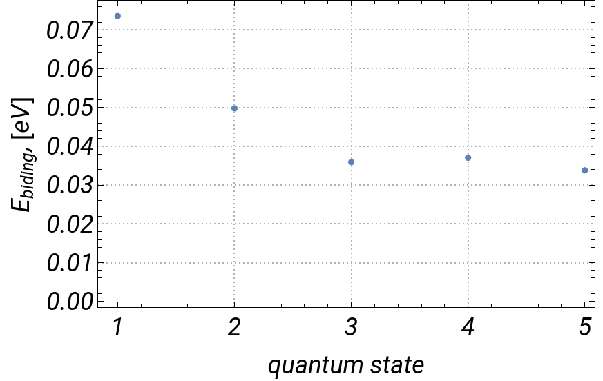
At first we can calculate the biding energy (the smallest amount of energy required to remove a particle from a system of particles or to disassemble a system of particles into individual parts). In our case, this is the difference between the energies when there is and is not an impurity.
Out[]=
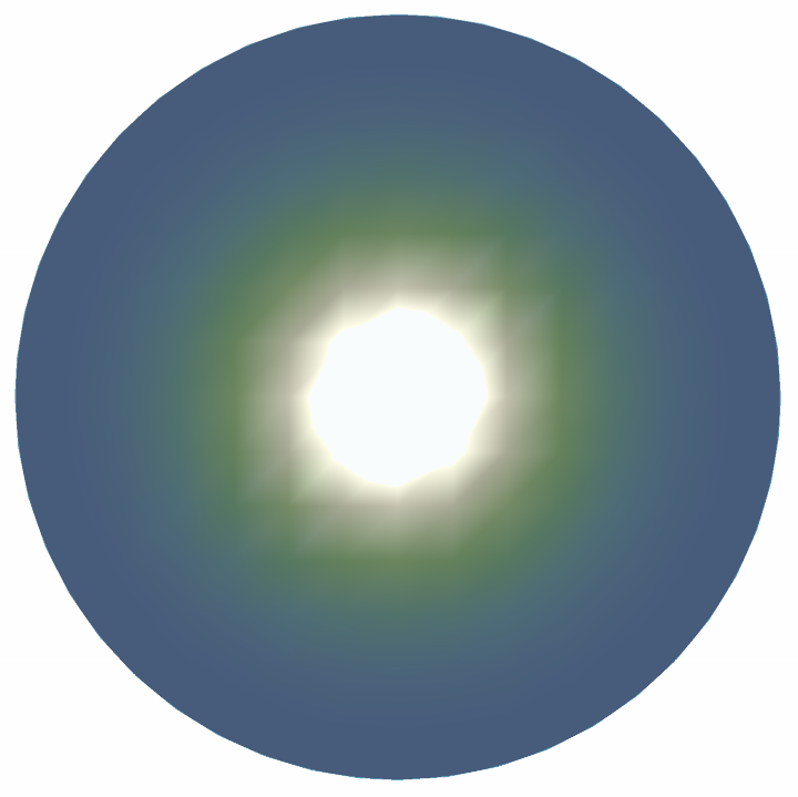
And finally, let’s imagine how it is possible to manipulate the location of an electron (electron cloud) by changing the location of an impurity (the coordinates of the impurity are determined by the locator).
Out[]=

CITE THIS NOTEBOOK
CITE THIS NOTEBOOK
Impurity states and density plots in quantum dots
by Khachik Khachatryan, M.A. Mkrtchyan
Wolfram Community, STAFF PICKS, May 4, 2025
https://community.wolfram.com/groups/-/m/t/3454665
by Khachik Khachatryan, M.A. Mkrtchyan
Wolfram Community, STAFF PICKS, May 4, 2025
https://community.wolfram.com/groups/-/m/t/3454665