Iteration Methods for Solving Kepler's Equation
Iteration Methods for Solving Kepler's Equation


After Johannes Kepler had discovered the equal area law of planetary motion, he tried to apply this law to determine the position of a planet in an elliptical orbit as a function of time. By ingenious geometrical manipulation, he reduced this task to what has become known as Kepler's problem: for any angle (the mean anomaly) and any number , determine an angle (the eccentric anomaly) such that Kepler's equation holds. Kepler was unhappy about not being able to find a closed-form solution and had to resort to numerical trial and error, with precomputed numerical tables providing a starting approximation.
M
e∈[0,1)
E
M=E-esinE
This Demonstration shows a contemporary version of Kepler's approach, an iterative algorithm that can solve the problem to any desired accuracy.
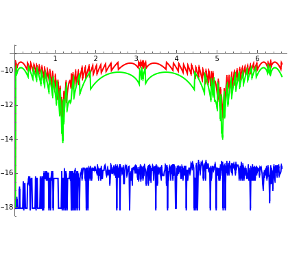
The values of form an equally spaced lattice on the axis. In each of the iteration methods considered, a value of is computed for each value of . With "timing", the cumulative computation times for the respective iteration methods are represented as a bar chart. For each iteration method, selecting "curves" shows one of three quantities as a function of : the value of , the number of iterations performed, and the absolute error .
M
x
E
M
M
E
|M-E+esinE|
Mouse over the control labels and graphics for full explanations.
Details
Details
Snapshot 1: The pure Newton iteration (notice "steps" is 0) shows excessive residual error for close to 1 (see peaks in the blue curve).
e
Snapshot 2: The Newton iteration preceded by three steps of averaged standard iteration yields tiny residual errors for all . Standard iteration (red curve) fails to reach the accuracy goal near .
e<1
M=π
Snapshot 3: This and the following snapshots deal with the larger eccentricity . Here we show the computation time for 5000 evaluations of for each of the three iteration methods. Due to the consistently low number of iterations, the Newton method (blue curve) is fastest.
e=0.9
E
Snapshot 4: All methods are seen to keep the residual error below the value (see ) set by the termination condition. But the Newton iteration underestimates this by about five orders of magnitude.
-9
10
p=-9
Snapshot 5: The large number of required iterations of standard iteration (red curve) explains that this method, although involving the simplest formula, is slowest.
Snapshot 6: The computed values of coincide for all iteration methods in graphical resolution.
E
Snapshot 7: This is no longer the case if we restrict the allowed iterations to a low value, such as 10 in the present case. Notice that by selecting and appropriately, we show the critical region around where standard iteration (red) asks for many iterations. Therefore, the error caused by restricting the number of iterations becomes visible.
x
L
d
M=π
Consider three different but interrelated iteration schemes. To formulate them compactly, abbreviate Kepler's equation as , where and are implicit parameters. The most obvious method, which works very well for, say, , is nesting function :
E=f(E)
M
e
e<0.2
f
(a) =f().
E
i+1
E
i
The next one is (a) with a simple provision against oscillation by averaging over two adjacent simple iteration results. This method seems not to be in common use:
(b) =f(), =f(), =(+).
E
⋆
E
i
E
⋆⋆
E
⋆
E
i+1
1
2
E
⋆
E
⋆⋆
It always converges, even for , but it needs many iterations if is near to an integer multiple of . The most sophisticated method is defined as a few steps (e.g. three steps) of method (b) followed by the Newton iteration:
e=1
E
2π
(c) =--f().
E
i+1
E
i
E
i
E
i
1-f'()
E
i
Running all methods with the same termination condition , the error in method (c) is orders of magnitude smaller than in methods (a) and (b). The Demonstration shows that method (c) definitively outperforms (b). The role of (b) thus becomes a robust and simple initialization method for the Newton iteration.
|-|<ϵ
E
i+1
E
i
|M-E+esinE|
Permanent Citation
Permanent Citation
Ulrich Mutze
"Iteration Methods for Solving Kepler's Equation"
http://demonstrations.wolfram.com/IterationMethodsForSolvingKeplersEquation/
Wolfram Demonstrations Project
Published: June 23, 2015