Convolutional Neural Networks are already being used to perform an increasing number of object identification challenges (CNN). Convolutional neural networks have improved most existing and new computer vision tasks because to their high recognition rate and quick execution. In this notebook, we propose to implement a convolution neural network to develop a traffic sign recognition system. In addition, this notebook compares and contrasts the existing “LeNet” Model with the customized enhanced model,this model gives 99.3% accuracy for 10 classes whereas it gives 97.1% accuracy for all classes when trained using GTSRB data.
Exploring GTSRB Data
Exploring GTSRB Data
◼
We will be using the GTSRB (German Traffic Sign Recognition Benchmark) data which has the following properties:-
Link for dataset - https://www.kaggle.com/meowmeowmeowmeowmeow/gtsrb-german-traffic-sign
◼ Single-image, multi-class classification problem
◼ More than 40 classes
◼ More than 50,000 images in total
◼ Large, lifelike database
Link for dataset - https://www.kaggle.com/meowmeowmeowmeowmeow/gtsrb-german-traffic-sign
◼ Single-image, multi-class classification problem
◼ More than 40 classes
◼ More than 50,000 images in total
◼ Large, lifelike database
This Data has three CSV files containing the paths of images and there are also respective folders containing the images which we will be using :-
CSVFiles | Folder |
test.csv | test |
train.csv | train |
meta.csv | meta |
◼
meta.csv
Contains the basic informations about the data.
Extracts the data present in “meta.csv” as a database format and after that it removes the unnecessary columns:
In[]:=
meta=Import["C:\\Users\\RAZORBLADE\\Desktop\\wolfram\\archive\\Meta.csv","Dataset","HeaderLines"1]
In[]:=
meta=SortBy[KeyDrop[{"ShapeId","ColorId","SignId"}]@meta,"ClassId"]
Extracts an image from “meta” folder using the path given by “meta” database:
In[]:=
GetClass[n_]:=Import[FileNameJoin[{$HomeDirectory,"Desktop","wolfram","archive",meta[[n+1,1]]}]]
◼
train.csv
Contains dataset for training.
Extracts the data present in “train.csv” as a database format and after that it removes the unnecessary columns.
In[]:=
train=Import["C:\\Users\\RAZORBLADE\\Desktop\\wolfram\\archive\\Train.csv","Dataset","HeaderLines"1]
In[]:=
train=KeyDrop[{"Width","Height","Roi.X1","Roi.Y1","Roi.X2","Roi.Y2"}]@train
We have around 40k images in training data.
In[]:=
Length[train]
Out[]=
39209
◼
test.csv
Contains dataset for testing.
Extracts the data present in “test.csv” as a database format and after that it removes the unnecessary columns.
In[]:=
test=Import["C:\\Users\\RAZORBLADE\\Desktop\\wolfram\\archive\\Test.csv","Dataset","HeaderLines"1]
In[]:=
test=KeyDrop[{"Width","Height","Roi.X1","Roi.Y1","Roi.X2","Roi.Y2"}]@test
We have around 13k images in test data.
In[]:=
Length[test]
Out[]=
12630
Processing the data for training and testing
Processing the data for training and testing
◼
In this section we will be seeing some difficulties with our data and then we will be processing our data for training and testing.
Before that, let’s see the distribution of different classes in our training data:-
Before that, let’s see the distribution of different classes in our training data:-
Classes just contains all the data from “ClassId” Column from train database in list format.
In[]:=
Classes=train[All,"ClassId"]//Normal
In[]:=
SortedClasses=SortBy[Tally[Classes],First]
In[]:=
BarChart[Apply[Labeled,Reverse[SortedClasses,2],{1}],AxesLabel{"ClassId","Amount of Data"},PlotLabel"Training Data Distribution",ImageSizeLarge]
Out[]=
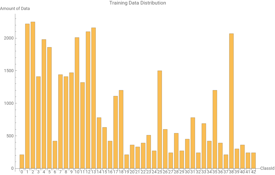
We have to reduce the number of classes to lower our training time. We will be considering only 10 classes, selecting the classes that have relevant differences.
Observing the above distribution , it has a relevant variance in the amount of images for each class for e.g. for Class-0 we have 210 images, while for Class-38 we have 2070 images. This is a problem called data unbalance, which can make the model learn only from the classes that have more data, and less from the others. To solve this problem we will be selecting 10 classes of which have approximately similar amount of data.
Observing the above distribution , it has a relevant variance in the amount of images for each class for e.g. for Class-0 we have 210 images, while for Class-38 we have 2070 images. This is a problem called data unbalance, which can make the model learn only from the classes that have more data, and less from the others. To solve this problem we will be selecting 10 classes of which have approximately similar amount of data.
Selects 10 classes.
In[]:=
FinalOutputClasses={8,10,11,12,13,14,17,18,25,38}
Out[]=
{8,10,11,12,13,14,17,18,25,38}
Process training dataset
Process training dataset
◼
Now, first we will shuffle and filter the train database such that it contains only those rows whose “Classid” value is present in the “FinalOutputClasses” by using “MemberQ” function an we will call the new database as “Finaldata”.
“FinalClasses” and “FinalLocations” are just list formats of the columns present in the “Finaldata” database.
“FinalClasses” and “FinalLocations” are just list formats of the columns present in the “Finaldata” database.
In[]:=
Finaldata=RandomSample[train[Select[MemberQ[FinalOutputClasses,#ClassId]&]]]
In[]:=
FinalClasses=Finaldata[All,"ClassId"]//Normal
In[]:=
FinalSortedClasses=SortBy[Tally[FinalClasses],First]
Out[]=
{{8,1410},{10,2010},{11,1320},{12,2100},{13,2160},{14,780},{17,1110},{18,1200},{25,1500},{38,2070}}
In[]:=
BarChart[Apply[Labeled,Reverse[FinalSortedClasses,2],{1}],AxesLabel{"ClassId","Amount of Data"},PlotLabel"Training Data Distribution",ImageSizeMedium]
Out[]=
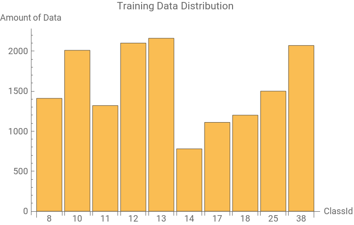
Above is the distribution for final training data
In[]:=
FinalLocations=Finaldata[All,"Path"]//Normal
The function “GetFile” gets the data present at address “s” .
In[]:=
GetFile[s_]:=Import[FileNameJoin[{$HomeDirectory,"Desktop","wolfram","archive",s}]]
Now Let’s get the final training data, for this we will first resize each image into 32*32 pixels because it is what we will be feeding into our model and make it as list of rules.
It will take few minutes.
It will take few minutes.
In[]:=
train1=Table[ImageResize[GetFile[FinalLocations[[i]]],{32,32}]->Position[FinalOutputClasses,FinalClasses[[i]]][[1,1]]-1,{i,1,Length[FinalClasses]}]
Processing our testing data
Processing our testing data
◼
“FinalTestClasses” and “FinalTestLocations” are just list formats of the columns present in the “FinalTestdata” database similar to what we did with the train database.
In[]:=
FinalTestdata=RandomSample[test[Select[MemberQ[FinalOutputClasses,#ClassId]&]]]
In[]:=
FinalTestClasses=FinalTestdata[All,"ClassId"]//Normal
In[]:=
FinalTestLocations=FinalTestdata[All,"Path"]//Normal
In[]:=
Datatobetested=Table[ImageResize[GetFile[FinalTestLocations[[i]]],{32,32}]->Position[FinalOutputClasses,FinalTestClasses[[i]]][[1,1]]-1,{i,1,Length[FinalTestClasses]}]
◼
Finally we have around 16k training data and 6k testing data so now we can work on our models.
Train Existing LeNet Model
Train Existing LeNet Model
Model Construction
Model Construction
First lets see the existing “LeNet” Model, from below output we can observe that this model have 4 types of Layers present in it.◼ Convolutional Layer - A convolutional layer is the main building block of a CNN. It contains a set of filters (or kernels), parameters of which are to be learned throughout the training. The size of the filters is usually smaller than the actual image. Each filter convolves with the image and creates an activation map. For convolution the filter slid across the height and width of the image and the dot product between every element of the filter and the input is calculated at every spatial position.◼ Pooling Layer - Pooling layers are used to reduce the dimensions of the feature maps. Thus, it reduces the number of parameters to learn and the amount of computation performed in the network.◼ Flatten Layer - It just convert 2d data to 1d to further feed on subsequent fully connected layers.◼ Softmax Layer - Softmax Layer assigns decimal probabilities to each class in a multi-class problem. Those decimal probabilities must add up to 1.0. This additional constraint helps training converge more quickly than it otherwise would.It comes before the output layer.All layers which are in red colour have learnable parameters.
In[]:=
NetModel["LeNet"]
Out[]=
NetChain


Training the model
Training the model
We can also see the details of any particular layer, let’s see details of layer 4 by below code which also describes the properties of this layer like Output Channels,KernelSize,Stride,Padding size etc.
OR
We can just click on the desirable layer of the NetChain to know more about it .
OR
We can just click on the desirable layer of the NetChain to know more about it .
Testing the model
Testing the model
◼
Now Lets test this model with our testing data using following code
We can see that this existing model worked well and is around 96.7% accurate on classifying the testing data.
Train Enhanced Model
Train Enhanced Model
Model Construction
Model Construction
◼
Now it is time to create our enhanced model such that we get accuracy larger than previous accuracy, but before that we have to configure our encoder and decoder .
“encoder” is the encoder which we are using here , it take an image as an input and outputs an array of size(3*32*32) see below.
“decoder” is the decoder which we are using here , it outputs the final class for which the probability is highest.
“encoder” is the encoder which we are using here , it take an image as an input and outputs an array of size(3*32*32) see below.
“decoder” is the decoder which we are using here , it outputs the final class for which the probability is highest.
Model Training
Model Training
Model Testing
Model Testing
◼
At last after training and testing , we can see that the accuracy has increased to 99.14% which is better than existing “LeNet” Model.
All Classes
All Classes
In this section, we will try to build a model to classify for all 43 classes.
Data for training
Data for training
◼
Now we know that our data distribution is not very good, so to solve this problem we will select around mean of the data from each classes for training which is also called as data downsampling.
Let’s calculate the mean first.
The below function “GetData[i]” returns the data for classId i depending on the amount of data it have which means it will return all data if it has less than mean amount of data whereas it will return randomly selected mean amount of data if it has more than mean amount of data.
Below is the new distribution.
Loc contains respective locations of all images for training
We will store our training data in “trainingData” list.
Below code collects all training data.
We have around 26k data for training.
Augmentation
Augmentation
◼
Another thing we need to do is augmentation.
◼
For this, we will rotate each image of all classes which have less than mean/2 number of images by 90 degree and add it to the training data.
Select all classes which have less than mean/2 number of images
Rotate each image by 90 degree and append it to the “trainingdata” list
Now Let’s get our testing data
Train Existing LeNet model
Train Existing LeNet model
Model Construction
Model Construction
◼
Let’s try to train using the existing LeNet model first and then we will move on the custom model.
◼
Note here that i have hard coded the “LeNet” model here unlike previous one.
Training the Model
Training the Model
Testing the model
Testing the model
So, we can see that the accuracy we get is around 93.5%.
Train Enhanced Models
Train Enhanced Models
Model Construction
Model Construction
◼
Now lets try the enhanced model which we used before and see the results.
Training the model
Training the model
Testing the model
Testing the model
So, from the above results we can say that the best accuracy we are getting is 97%
Concluding remarks
Concluding remarks
◼
We have seen that for classifying only 10 classes , accuracy was higher (99%) than classifying with all classes (97%) and there are many reasons behind like no of output nodes, quality of data, amount of data for training etc.
Another important thing to note is that it is very important to explore more than just one model to get the best accuracy.
For the second case, the accuracy can still be increased by performing some other complex image manipulations like Contrast Limited Adaptive Histogram Equalization (CLAHE) and training it with the model .
Another important thing to note is that it is very important to explore more than just one model to get the best accuracy.
For the second case, the accuracy can still be increased by performing some other complex image manipulations like Contrast Limited Adaptive Histogram Equalization (CLAHE) and training it with the model .
Keywords
Keywords
◼
CNN
◼
GTSRB
◼
Image Classification
Acknowledgment
Acknowledgment
I would like to thank my mentor Siria Sadeddin for solving my doubts regarding the project.
I would also like to thank Swatik Banerjee and Rahul Sharma for their help.
I would also like to thank Swatik Banerjee and Rahul Sharma for their help.
References
References