Large Language Models (LLMs) have demonstrated their strong capabilities in language modelling, text generation, and many other natural language understanding tasks compared to their predecessors. We hypothesize LLMs gain their strength by successfully mapping words onto the semantic space, and traversing through the semantic space with high degree of stability. We model the computation of LLMs as trajectories in their embedding space. We study the stability of the trajectory by introducing small amount of controlled noise into the input word embeddings. We demonstrated that GPT3 are more capable of resisting small perturbations in the input space compared to GPT2 model.
We start with investigating GPT2 model [1] provided by Wolfram Neural Net Repository. The model is pre-trained on WebText data. we will use version with 117M parameters for our experiments, though the same workflow can easily be extended to versions with larger parameter size.
The input sentence is first converted into a sequence token. The stream of token is then converted to a n by 768 matrix through both positional embedding layer and token embedding layer. The output from embedding layer is then fed into the decoder module, which is the major component of the model. It consists of 12 self-attention modules that independently read/write informations from/to the residual stream. The output of the decoder is a n by 768 matrix. We feed the last row of this matrix to linear classifier layer which output the probability distribution over tokens through a softmax layer.
The input sentence is first converted into a sequence token. The stream of token is then converted to a n by 768 matrix through both positional embedding layer and token embedding layer. The output from embedding layer is then fed into the decoder module, which is the major component of the model. It consists of 12 self-attention modules that independently read/write informations from/to the residual stream. The output of the decoder is a n by 768 matrix. We feed the last row of this matrix to linear classifier layer which output the probability distribution over tokens through a softmax layer.
In[]:=
gpt2lm
Out[]=
NetChain


Similarity matrix for concept space mapping
Similarity matrix for concept space mapping
To gain a understanding on the structure of the semantic space, we first explore what are the similar embedding in this space. Note that its impossible to enumerate all possible token sequence, therefore we choose to take a specific example that will be used later in this notebook.
The successive phrases for a sentence “The man speaks French, he is from the city of” is defined as the following
Out[]=
The |
The man |
The man speaks |
The man speaks French |
The man speaks French, |
The man speaks French, he |
The man speaks French, he is |
The man speaks French, he is from |
The man speaks French, he is from the |
The man speaks French, he is from the city |
The man speaks French, he is from the city of |
We then feed each of these successive phrases into the GPT2 and GPT3 (text-embedding-ada-002) to obtain the 768 dimensional embedding vector for GPT2 and 1536 dimensional vector for GPT3. When then calculate pairwise cosine similarity between them and plot them as heatmap as following.
In[]:=
With[{sentence="The man speaks French, he is from the city of"},Row[{subsentenceSimilarity[sentence,PlotLabel->"GPT2",ImageSize->330],subsentenceSimilarityGPT35[sentence,PlotLabel->"GPT3",ImageSize->330]}]]
Out[]=
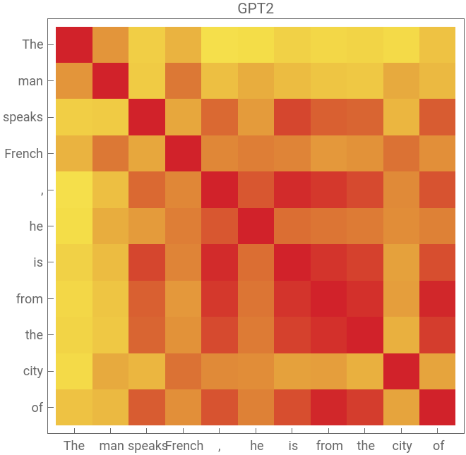
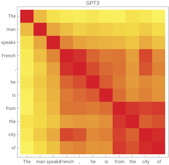
It is interesting to see the segregated structure shown in GPT3’s similarity plot. After the model sees token “French”, every subsequent phrases are comparatively similar. The same situation happens when models sees the token “from”. The similarity matrix plot for GPT2 did not demonstrate the same pattern. A few more examples with different sentence are shown at the end of the notebook.
We hypothesize that GPT3 model implicitly learns to segregate the embedding space into hierarchies of contextualized spaces, where it learns to progressively switch to more specific contexts following the input sequence. A more detailed study in the future is needed in the future to confirm our hypothesis.
We hypothesize that GPT3 model implicitly learns to segregate the embedding space into hierarchies of contextualized spaces, where it learns to progressively switch to more specific contexts following the input sequence. A more detailed study in the future is needed in the future to confirm our hypothesis.
Now, what are the small changes we can make in the embedding layer? Our solution is to add scaled unit normal noise.
Random noise at embedding
Random noise at embedding
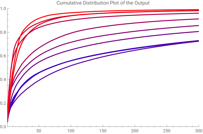
We first experiment with adding random noise to the embedding and observe the output distribution. The random noise are generated from the unit normal distribution, and scaled according to the noise level α, the following plot shows the cumulative distribution of the output w.r.t. different α value. Tokens on x axis is sorted in descending order according to their probabilities. Each plot are averaged over 10 trials.
It seems the model is more confident when there are more noise introduced into the embedding. And the confidence level does not scale linearly w.r.t. the level of noise added to the embedding. There is a gap between α=0.8 and α=1.4. The GPT2 model seems to be resistant to noise level up to α=0.4
It seems the model is more confident when there are more noise introduced into the embedding. And the confidence level does not scale linearly w.r.t. the level of noise added to the embedding. There is a gap between α=0.8 and α=1.4. The GPT2 model seems to be resistant to noise level up to α=0.4
Out[]=


It is interesting to study the embedding space of the sentence, however it also comes with a few issues. Firstly, the noise added does not go through decoder, which is the most important component of the model. And most importantly, there isn’t a good way to propagate the noise signal back to the neural network because it can only take a sequence of token as inputs. Therefore, we decided it would be more interesting to take a look at the perturbation at word embedding level.
Footnote:
Interpolating token embeddings
Interpolating token embeddings
There are a couple of advantages interpolating token embeddings. The space of input are drastically reduced to 50k tokens, and more importantly, distance measurements are intrinsic part of the human perception, We can immediately tell that the word “dog” and “cat” are semantically closer that “dog” and “spacecraft”. Therefore, we can control the change introduced into the token embedding space by interpolating between token embedding vectors.
We have also measured the KL divergence between the output distribution throughout the interpolation. We fix a origin token in this case “ French”, and interpolate it to different tokens, some of them are semantically closer in human perception while others are farther away.
Out[]=
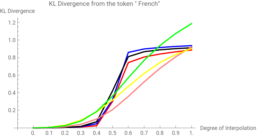


There seems to be a general trend that semantically closer (under human perception) tokens results in smoother output distribution by the model. One possible interpretation is that models are taught to always stick with the semantic meaningful regions in the embedding space. If the interpolation leads to travelling between two semantically meaningful space, then it would be best to quickly travel through the semantically meaningless region in the middle, which leads to the seemingly sudden transition in the output distribution.
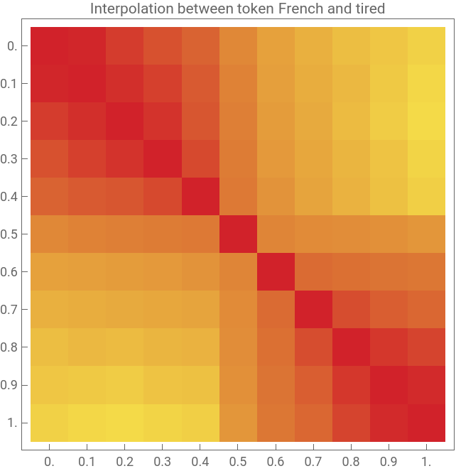
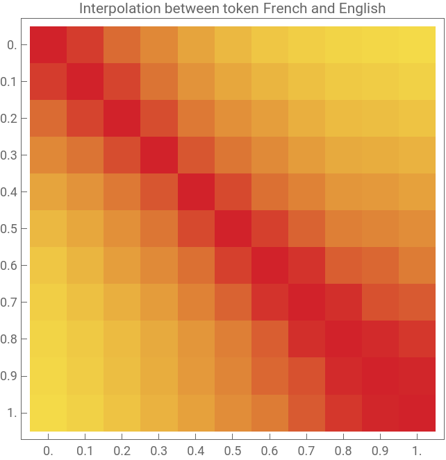
Now lets take a more detailed look at the transition between semantic spaces. For a pair of token, in this example “ French” and “ English”, we can calculate the interpolated token embedding vector, and then feed it into the model to obtain the sentence level embedding vector. We then calculate pair-wise cosine similarity for all sentence level embedding vectors.
The left side figure represent the interpolation between token “ French” and token “ biscuits”, and the right side figure represents the interpolation between “ French” and “ English”.
It is interesting that we can see a sharper transition between the conceptual space from “ French” to “ biscuits” than from “ French” to “ English”. It is a indicator that there may be discontinuation from the concept space of “ French” to “ biscuits”.
Out[]=
Footnote:
Trajectories in the embedding space
Trajectories in the embedding space
Now lets try to get a global view on how does GPT model move it the embedding space.
Here we show the trajectories of the GPT2 in its embedding space. Each blue point corresponds to the a embedding vector of one of the successive phrases. The red spheres correspond to the 10 most likely tokens predicted by the GPT2 with their size scaled according to the probabilities, their embeddings are also whole sentence embedding to make them comparable with the trajectory embeddings. The trajectory corresponds to the sentence “The man speaks<slot>, he is from the city of”, each of the 4 figures corresponds to different language inserted at <slot>.
In general, GPT2 seems to be making quite sensible decisions. For example, when the input word is “French”, it correctly predicted “Marse” and “Paris”. And in most cases, there are clear separations between character tokens and whole word tokens.
The general trajectories of GPT2 does seems to relatively stable under linear transformations. However, the relative position between the predicted embedding and trajectories embeddings make the trajectory plot looks chaotic.
Out[]=
 |  |
 |  |
However, for GPT3 the trajectory is much more stable. The perturbation did not change the general direction of the trajectory.
And compare to GPT2, GPT3 seems to provide better contextualization compared to GPT2. For example, the embedding of the second “he” is quite far away from the first “He” for GPT3, but the same cannot be said for GPT2. This also matched our observation in the similarity heatmap example.
And compare to GPT2, GPT3 seems to provide better contextualization compared to GPT2. For example, the embedding of the second “he” is quite far away from the first “He” for GPT3, but the same cannot be said for GPT2. This also matched our observation in the similarity heatmap example.
Out[]=
 |  |
 |  |
The comparison is even more obvious when we use a more complicated sentence.
The general trajectory of GPT2 seems to break down completely when we use meaningless character to fill the slot, but the trajectory of GPT3 seems to remain stable.
The contrast is the most apparent when when put GPT2 and GPT3 side by side.
Concluding remarks
Concluding remarks
Large Language Models are becoming critical tools for improving general human productivity, yet our understanding of the internal workings of these models remains limited. From GPT2 to GPT3 and GPT4, intelligent behaviour seemingly arise from pure scaling of the model size, training data and slight modification of tokenization scheme.
In this project, we compared the GPT2 and GPT3.5 model to investigate their trajectories in the embedding space. We found that GPT3.5 is much more stable under small perturbations. And a possible cause for such stability might come from its capability for contextualization.
In this project, we compared the GPT2 and GPT3.5 model to investigate their trajectories in the embedding space. We found that GPT3.5 is much more stable under small perturbations. And a possible cause for such stability might come from its capability for contextualization.
Some of potential future extensions of this work includes the following
◼
our works are mostly qualitative. To concretize our claim, more quantitative study on the embedding trajectories is needed. It is possible to leverage methods from numerical analysis along with some existing mathematical formulations of transformer architecture to gain insights into the nature of decision making process of LLMs.
◼
part of our study are not applicable due to the close-source nature of GPT3.5/GPT4 model. If in the future OpenAI decide to make them open source, it should be fairly easy to apply the same workflow to them.
◼
To construct the visualization in 2/3D, we used DimensionReduce function, which essentially applies Principle Components Analysis (PCA) on the input n by 768 matrix. A possible extension is to extract the variance explained by the dimension reduction method and perform different dimension reduction techniques.
◼
In this project, we chose to focus on a limited selection of sentences to reduce the space of inputs. However, in principle the work can be easily extended to a vast array of sentences, examples include prompts being submitted to Wolfram Prompt Repository.
◼
In the interpolation section, we chose to interpolate a pair of single tokens. A possible extension is to interpolate between N singular tokens.
In conclusion, there are many more works to be done in understanding LLMs. By computationally evaluate critical structures in LLMs, we hope to promote further study in the science of LLM, and ultimately harness the power LLMs in advancing various domains and industries.
Keywords
Keywords
◼
Large language model
◼
Generative pretrained transformers
Acknowledgment
Acknowledgment
I would like to thank Bob Nachbar, Christopher Wolfram, Jofre Espigule and Mark Greenberg for their invaluable guidance in the overall development of the project. I am grateful to Stephen Wolfram for providing the initial idea that inspired this project. Additionally, I want to extend a special thanks to my mentor Alejandra Ortiz for carrying me throughout the project (and possibly burned down her laptop for running some heavy-lifting computation).
References
References
◼
[1] A. Radford, J. Wu, R. Child, D. Luan, D. Amodei, and I. Sutskever, “Language Models are Unsupervised Multitask Learners”.
CITE THIS NOTEBOOK
CITE THIS NOTEBOOK
Study the effect of small changes in large language models
by Luhan Cheng
Wolfram Community, STAFF PICKS, July 12, 2023
https://community.wolfram.com/groups/-/m/t/2958873
by Luhan Cheng
Wolfram Community, STAFF PICKS, July 12, 2023
https://community.wolfram.com/groups/-/m/t/2958873