Dynamics of a binary distillation column
Authors: Housam Binous and Ahmed Bellagi
Dynamics of a binary distillation column
Authors: Housam Binous and Ahmed Bellagi
Authors: Housam Binous and Ahmed Bellagi
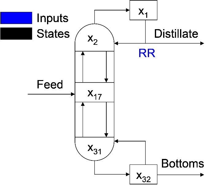
A dynamic simulation of a distillation column with 32 stages is performed . We consider that the relative volatility of the binary mixture is constant equal to 1.6 . We find the steady state mole fractions in all stages when the reflux ratio is equal to 3. Then, we perform a step in the reflux ratio (i . e . we take a reflux ratio equal to 1.5 or 4.5) . We plot the dynamic behavior of the mole fractions in all stages .
Application: The dynamic behavior when we submit the column to a step in the reflux ratio allow us to obtain transfer functions, which are key in process control simulations of distillation columns.
In a similar fashion, one can also perform dynamic simulation using positive or negative steps in the reboil ratio, reboiler heat duty... However, derivation of the full MESH equations (obtained from mass and energy balances, phase equilibrium relations and mole fractions summations) may be required.
Note that this simulation based on constant relative volatility assumption will not allow you to have access to the temperature profile inside the column.
Acknowledgment: This computation was inspired from a Matlab program available at the Nonlinear Model Database by John Hedengren ( Brigham Young University). Link: http://www.hedengren.net/research/models.htm
In[]:=
Off[General::"spell"]
We consider a binary mixture with constant relative volatility α=1.6For a binary mixture with constant relative volatility, the equilibrium equation writes:
y=
αx
1+(α-1)x
In[]:=
α=1.6;
In[]:=
Table[y[i_,t_]:=x[i,t]*α/(1+(α-1)*x[i,t]),{i,1,32}];
The governing equations below are merely the component material balance equations
Governing equations in the rectifying section .
In[]:=
eq[1]=D[x[1,t],{t,1}]1/hdcondV(y[2,t]-x[1,t]);
In[]:=
eq[i_]:=D[x[i,t],{t,1}]1/hdup(L(x[i-1,t]-x[i,t])-V(y[i,t]-y[i+1,t]))
Governing equations in the feed stage
In[]:=
eq[17]=D[x[17,t],{t,1}]hdup(FxF+Lx[16,t]-Lpx[17,t]-V(y[17,t]-y[18,t]));
Governing equations in the stripping section
In[]:=
Eq[i_]:=D[x[i,t],{t,1}]1/hdup(Lp(x[i-1,t]-x[i,t])-V(y[i,t]-y[i+1,t]))
In[]:=
Eq[32]=D[x[32,t],{t,1}]1/hdreb(Lpx[31,t]-(F-Dist)x[32,t]-Vy[32,t]);
Feed flow rate and composition
In[]:=
xF=0.5;
F=24/60.;(*expressedinmol/min*)
Molar hold up in the reboiler, condenser and trays
In[]:=
hdreb=1.0;
In[]:=
hdup=0.25;
In[]:=
hdcond=0.5;
Reflux ratio, Distillate flow rate, Liquid and vapor flow rates in both sections of the column
Vp and Lp are the vapor and liquid flow rate in the stripping section, respectively.
V and L are the vapor and liquid flow rate in the rectifying section, respectively.
Because the thermal quality of the feed is taken to be saturated liquid, we have Lp=L+F and Vp=V
Vp and Lp are the vapor and liquid flow rate in the stripping section, respectively.
V and L are the vapor and liquid flow rate in the rectifying section, respectively.
Because the thermal quality of the feed is taken to be saturated liquid, we have Lp=L+F and Vp=V
In[]:=
Dist=0.5F;
In[]:=
L=R*Dist;
In[]:=
Lp=F+L;
In[]:=
V=L+Dist;
In[]:=
R=3;
Steady state for R=3.0
In[]:=
sol=NDSolve[Join[{eq[1]},Table[eq[i],{i,2,16}],{eq[17]},Table[Eq[i],{i,18,31}],{Eq[32]},Table[x[i,0]0.5,{i,1,32}]],Table[x[i,t],{i,1,32}],{t,0,20000}]
Out[]=
Liquid-phase composition versus stage number in the column
In[]:=
Table[x[i,t]/.sol/.t20000,{i,1,32}]
Out[]=
{{0.935419},{0.900526},{0.862296},{0.821699},{0.779991},{0.738572},{0.698805},{0.661843},{0.628508},{0.599253},{0.574186},{0.553144},{0.535785},{0.521665},{0.510315},{0.501275},{0.494129},{0.48545},{0.474203},{0.459803},{0.441645},{0.419187},{0.392063},{0.360231},{0.324105},{0.284637},{0.243266},{0.201745},{0.161848},{0.125085},{0.0924957},{0.0645806}}
In[]:=
TableForm[Table[{i,x[i,t]/.sol/.t20000},{i,1,32}]]
Out[]//TableForm=
1 |
| |
2 |
| |
3 |
| |
4 |
| |
5 |
| |
6 |
| |
7 |
| |
8 |
| |
9 |
| |
10 |
| |
11 |
| |
12 |
| |
13 |
| |
14 |
| |
15 |
| |
16 |
| |
17 |
| |
18 |
| |
19 |
| |
20 |
| |
21 |
| |
22 |
| |
23 |
| |
24 |
| |
25 |
| |
26 |
| |
27 |
| |
28 |
| |
29 |
| |
30 |
| |
31 |
| |
32 |
|
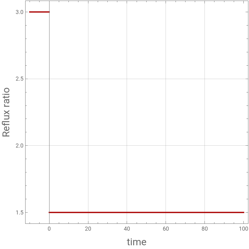
Perform a negative step in the reflux ratio (take R=1.5).
In[]:=
R=1.5;
In[]:=
Plot[3-1.5UnitStep[x],{x,-10,100},Frame->True,GridLines->Automatic,FrameLabel->{Style["time",16],Style["Reflux ratio",16]},AspectRatio->1,ImageSize->400{1,1},PlotStyle->{Thick,Darker@Red}]
Out[]=
In[]:=
sol2=NDSolve[Join[{eq[1]},Table[eq[i],{i,2,16}],{eq[17]},Table[Eq[i],{i,18,31}],{Eq[32]},Table[x[i,0]x[i,t]/.sol/.t20000,{i,1,32}]],Table[x[i,t],{i,1,32}],{t,0,20000}]
Out[]=
In[]:=
Plot[Evaluate[Flatten[Table[x[i,t]/.sol2,{i,1,16}]]],{t,0,60},PlotStyleTable[Hue[i/33],{i,1,16}],PlotRange{0.45,1},Frame->True,AspectRatio->1,GridLines->Automatic,FrameLabel->{Style["time",16],Style["Liquid-phase composition in the rectifying section",16]},ImageSize->400{1,1},PlotLegends->Table[i,{i,1,16}]]
Perform a positive step in the reflux ratio (take R=4.5).