Abstract: This project investigates the relationship between cellular automata and regular languages. The primary objective is to determine outputs that cannot occur from any input in a given cellular automaton characterized by the number of states (k), and neighborhood radius (r). This can be done by constructing and analyzing De Bruijn graphs. Each graph will be annotated with a particular cellular automaton’s transition rules, either with a Moore or Mealy machine structure. The machines can be transformed into a deterministic form where the question of missing inverses reduces to path finding on a directed graph.
Initialization
Initialization
1. Introduction
1. Introduction
1.1: Introduction & Definitions
1.1: Introduction & Definitions
1.1.1: Cellular Automaton
1.1.1: Cellular Automaton
Cellular automata could be thought as simple mathematical idealizations of natural systems.
They consist of a grid of identical discrete sites, each of which can take on a finite set of integer values. The values of these sites change in discrete time steps based on deterministic rules that determine the value of each site by considering the values of neighboring sites. As such, cellular automata could be seen as systems that evolve in discrete transition steps, following the steps indicated by a deterministic set of transition rules.
Consider the following automata described by this production rules:
Out[]=
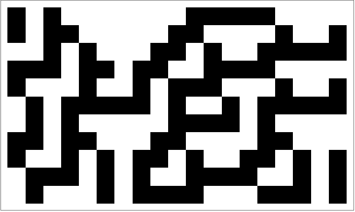
Then, the evolution of an initial state could be constructed just following the given rules of production:
In[]:=
ArrayPlot[CellularAutomaton[30,{1,0,1,0,0,0,0,0,0,0,1,1,1,1,1,0,0,0,0},10]]
Out[]=
In[]:=
ArrayPlot[CellularAutomaton[30,{{1},0},50]]
Out[]=
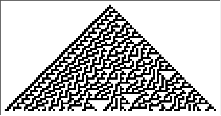
It is clear that, if only the transition rules are known, it would not be easy to determine if there are impossible blocks in automata outputs. In fact, the expansion in complexity describing these systems could even invite to think that there are no impossible blocks.
As a counterexample of this idea, consider the next automaton:
Out[]=
Is it possible for this automaton to produce an output that contains a black square? The answer is clear.
In this project, this question will be explores from a more general perspective and a method to determine these impossible blocks will be provided without having to compute transitions from the cellular automata.
The description of a one-dimensional cellular automaton requires three elements: rule identifier integer, an alphabet of possible states and a neighborhood radius value . With these considerations, transition rules can be thought as a function that allows as to determine the state of the i-th cell of the automaton at time step t, denoted by :
S{0,1,...,k-1}
r
ϕ:S
2r+1
S
(t)
a
i
Out[]=

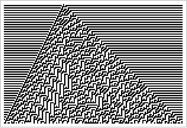
Here the transitions of rule 15 are included after 40 iterations (recall that k=2, r=1):
Out[]=

With the notation presented, one can consider that any general set of rules maps an initial configuration from the set of all possible configurations for the automaton to a new configuration in the same set. This function does not necessarily have to be onto; in this work, we show that there are non-possible blocks for the output set of an automaton.
Φ
A
0
Σ
A
1
Out[]=
Since there are possible input chain configurations on which a set transition rule can be applied, transition rules sets are needed to describe all cellular automata for fixed values of k and r.
2r+1
k
2r+1
k
k
The convention to assign an integer that identifies each automaton should be discussed. Each input string of symbols can be associated with the representation of an integer in base k (Since each symbol in this string takes values between 0 and k-1, this makes sens). The strings of input are sorted in descending order based on the integer represented by each. Then, each production rule generates a new state between 0 and k-1. Taking the values produced by each of the input strings results in a new string of symbols between 0 and k-1. This can also be a representation of an integer in base k, and this integer will be the identifier that represents the automaton.
2r+1
2r+1
k
Here are the 256 one-dimensional cellular automata with k=2, r=1. Each rule is associated with a digit in the base 2 representation of the integer identifier of the rule.
Out[]=


1.1.2: Mealy Machine
1.1.2: Mealy Machine
Finite-state machines are abstract models of machines with a primitive internal memory. A finite-state automaton is a special kind of finite-state machine that is closely linked to a particular type of language (both for input and output productions). Discrete mathematics and theory of computation frequently study these abstract models. In this post, we will explore two particular types of machines to describe cellular automata: Mealy and Moore machines.
Different types of machines that are classified according to different factors are examined, one of these is the existing relationship between output symbols, states and input symbols.
A Mealy machine is a machine in which the output symbol depends on the current input symbol and the current state of the machine.
This can lead to think that the transition graph of this machine contains information on the transition rule of the machine in the edges of the same and not only in the
vertices. This potential in to encode information on the vertices is what will be used for the construction of a graph that represents the rule of a cellular automata.
vertices. This potential in to encode information on the vertices is what will be used for the construction of a graph that represents the rule of a cellular automata.
1.1.3: Moore Machine
1.1.3: Moore Machine
A Moore Machine is a finite-state machine whose outputs depend on only the present state. This represents an important contrast to a Mealy machine, whose output depends by the current state and the input values.
This property invites to think that the transition information could be stored only in the vertices of the transition graph associated with a Moore Machine. This property will also be used when building another version of the graphs associated with cellular automata.
2. Automaton to a Graph: Part I - Mealy Machine
2. Automaton to a Graph: Part I - Mealy Machine
2.1: Non-Deterministic Mealy Machine
2.1: Non-Deterministic Mealy Machine
As an example to introduce this idea, consider the Non-Deterministic transition graph for a Mealy Machine associated to the one-dimensional cellular automaton with rule 76, k=2 and r=1:
The rules of production for this automata are:
This type of graph is called De Bruijn graph, named after the Dutch mathematician who utilized them to represent all possible sequences of symbols that can be generated within a language from a specified set of symbols.
To construct a graph, we begin with the premise that every production rule involves three digits: one central and two neighboring digits. In the graph, we can place two of these digits at the vertices, with the transition rule represented by the edge between them. Each vertex represents a pair of digits, and because every pair shares one digit with its neighboring vertices, the graph captures all possible overlaps between pairs of adjacent sequences.
For instance, a red edge connecting vertices 11 and 10 in the graph represents by overlap an input sequence of 110. According to the automaton’s description, this produces a 1, hence it is colored red. Conversely, the edge connecting 10 and 00, forming an overlap corresponding to input sequence 100, is colored black as it produces a 0 based on the automaton’s rule.
This graphical representation efficiently encapsulates the complete set of sequences derivable from a given set of symbols, illustrating the relationships and transitions between them.
Here there are more examples of this Mealy Machine graphs:
Rule 232 with k=2, r = 1:
Rule 0 with k=2, r=1:
Rule 10000 with k=2, r=2:
Rule 10000, k = 3, r = 2:
Rule 999, k = 2, r = 4:
The same graph, but without labeling:
Rule 999, k = 4, r = 2:
Examining the structure of several of these graphs reveals that most, if not all, of them are nondeterministic. This can be seen in the fact that for some vertices, there may be two different vertices whose edges have the same production value, for example, for rule 76, the vertex 10 can produce a 0 overlapping with 00 and 01 (100 and 101 produces 0 in that rule). There is a process to convert this non-deterministic machine into a deterministic one, where our objective of finding non-possible blocks in outputs could be reduced to path finding.
2.2: Deterministic Mealy Machine
2.2: Deterministic Mealy Machine
As mentioned in the previous section, generating the transition graph of an automaton thought of as a Mealy Machine provides a non-deterministic description of the automaton. It is convenient to transform this machine into a deterministic one. Based on the following theorem, this will always be possible to do:
Theorem:
Transformation of a nondeterministic finite-state automaton to a deterministic finite-state automaton
Transformation of a nondeterministic finite-state automaton to a deterministic finite-state automaton
The function presented in the previous section is used to construct the graph of the nondeterministic machine:
First, we separate the edges of the original graph by the production associated to them:
It will also be necessary to associate each vertex with all those vertices to which it can be related:
The last element needed to this construction is the power set of the vertices:
Now, the edges of a deterministic Mealy machine graph are generate using the association of edges and vertices, the association o vertices and this power set.
Since the original graph had 4 possible states, where all of them could be initial, now, in this new graph, the initial state is unique and must be the vertex that contains all the vertices of the nondeterministic graph.
We can note that this new graph is deterministic, since each vertex has only one incident edge associated with the production of a 0 and one incident edge associated with the production of a 1. The vertex e represents the empty set. If there is some vertex v connected to e can be understood as that there is no way that, being in any of the states included in v, it can produce the value associated with the edge connecting v with e. In this example, the vertex (1 1), can never produce a 1, so its connected to e with an edge that has a value of 1, the same happens with the vertex (0 1, 1 1).
Notice that some of the vertices of this graph have no edges arriving to them, this implies that these states cannot be reached from the initial state, so we can eliminate them and have a simpler graph.
Deterministic conversions of other rules are also included, also for k=2, r=1:
Rule 76:
Rule 255:
Rule 232:
Now, all the productions of this cellular automaton are summarized in all the possible paths that emerge from the initial state and do not reach e. Therefore, all the paths that emerge from the initial vertex and reach e are productions that can never be reached in this cellular automaton, so they will be impossible blocks in the chains produced by this automaton.
2.3: Non-Possible Blocks
2.3: Non-Possible Blocks
Based on the final discussion of the previous section, it is possible to determine the impossible blocks for the outputs of a cellular automata only by considering the graph of the deterministic Mealy machine associated with that automata. Consider again the example of rule 34 with k = 2, r = 1.
Paths that connect the initial state and e can be easily found and mapped to edge weights to determine which strings cannot be produced.
Finally, these non-producible strings are the following cellular automata output blocks:
This process can be replicated for all one-dimensional cellular automata regardless of the number of states or the radius of neighbourhoods. The theorem presented above assures us that it will always be possible to find a Mealy Machine equivalent to the one originally represented by the automaton.
Here are presented all the impossible blocks in outputs of the one-dimensional cellular automata with k=2, r=1 obtained using this method.
It is interesting that all multiples of 15 have no non-possible blocks.
3. Automaton to a Graph: Part 2 - Moore Machine
3. Automaton to a Graph: Part 2 - Moore Machine
3.1: Non-deterministic Moore Machine
3.1: Non-deterministic Moore Machine
Similar to constructing the state transition graph of a Mealy Machine, the behavior of a cellular automaton can also be described using the structure of a Moore Machine.
Unlike the previous case, where transition information is stored in the edges, here the information for each state is located in the vertices. The edges only contain information about the possible transitions connecting the states.
This construction is more explicit than in the previous case: the combinations of input strings are simply generated and the production information associated with each input is saved in the vertex weight.
Below are some examples of these types of graphs. CATransducer resource function was used to generate them:
This graph corresponds to Rule 76 and follows the same color scheme defined in the Mealy Machine examples: red indicates the production of 1, and black stands for the production of 0. Using this method, graphs with different states and neighborhoods can be generated, similar to those for the Mealy Machine.
Rule 167, k= 2, r = 2:
Rule 76, k = 3, r = 2:
3.2: Deterministic Moore Machine
3.2: Deterministic Moore Machine
To identify impossible blocks in outputs using the Moore Machine approach, we need the graph to be deterministic, just as in the case of Mealy Machines. The conversion process is similar, with the main difference being that the focus is now on the vertices, where the transition rule information is stored. Nevertheless, the theorem presented in Section 2.2 ensures the existence of a deterministic machine equivalent to any that can be generated by a cellular automaton.
The deterministic equivalent of this graph can be also constructed using an association of vertices according to the production associated with them and the vertex power set.
Here there are other examples of deterministic versions of the Moore machine graphs:
3.3: Non-Possible Blocks
3.3: Non-Possible Blocks
Now, we apply the same method to search for paths from the initial states to the vertex representing the empty set, which corresponds to impossible blocks in outputs.
Possible Initial States:
In this implementation, since the information is stored in the vertices, instead of using e for the empty set, we use {} and a label of the state that is produced by a transition to this vertex:
Pathfinding from the initial states to end states provides de trajectory that represents a non-possible block:
After mapping each path using the weights of the vertices to determine the production associated with them, we obtain the same solution:
Compare with the obtained using the previous method:
4. Automaton to a Graph: Part 3 - Discussion
4. Automaton to a Graph: Part 3 - Discussion
While it is true that both approaches yield similar results, it is evident that their different constructions lead to distinct complexity considerations.
4.1: Vertices and Edges
4.1: Vertices and Edges
Given that the transition graph information of a Mealy Machine is stored on the edges, it will require fewer vertices compared to a Moore Machine transition graph, which stores information about transition rules in the vertices.
This difference has significant implications for constructing the equivalent deterministic graph in each case, as it requires building a power set with all the vertices, which can be costly for a large number of vertices.
4.2: Visualization
4.2: Visualization
Despite the operational advantages of the transition graph of a Mealy Machine, it is important to note that working with graph structures provides grater visual control over what is happening in a given system. In this regard, it is also important to mention that due to the reduced number of vertices, the transition map representing a Mealy Machine transition graph is not necessarily easy to comprehend, and storing information on the edges complicates the labeling of the graph without interrupting other edges.
On the other hand, the transition graph of a Moore Machine clearly provides transition information at each vertex, making it easier for the reader to follow. Additionally, labeling is always less cumbersome when placed on the vertices.
Therefore, despite the efficiency discussed in the previous section regarding Mealy Machines, if working with small values of k and r, it is likely that a better visualization tool is provided by Moore Machines. In any case, both approaches are valid and have been observed to yield similar results when identifying impossible blocks for the outputs of cellular automata.
4.3: Different non-possible blocks
4.3: Different non-possible blocks
While it is true that up to this point, examples have shown that both methods find equivalent solutions, it is important to note that there are scenarios where this is not the case.
The explanation for this occurrence can be found in the different structures of the graphs. Due to their distinct constructions, the path-finding method will not necessarily find the same paths in bot graphs. Nevertheless, the solutions provided by both methods do correspond to impossible blocks. Therefore, two methods have been found that identify impossible blocks, and while they are conceptually equivalent, further review is required to conclusively affirm their complete equivalence.
Rule 76:
Rule 232:
Concluding Remarks
Concluding Remarks
The possibility to address the question of impossible blocks for a cellular automaton through transition graphs linked to deterministic Mealy or Moore machines simplifies the complexity associated with their evolution, reducing the problem to searching for impossible blocks in a directed graph. This approach to the problem proves successful for one-dimensional automata with two states and neighborhood radius ranging from 1 to 2. For larger radii and numbers of states, it becomes a computationally intensive exercise involving significant calculation time.
The Moore machine approach may offer a more visually intuitive representation of the automaton in a graph but requires a greater number of vertices and edges to operate effectively. The advantage of using a Mealy machine lies in the information stored in the edges, which reduces the number of vertices required.
Future Work
Future Work
Although significant results have been presented for one-dimensional cellular automata with k=2 and r = 1, it is important to note that the methods presented are valid for any value of k and r. The only drawback of these methods is computational complexity. Given exponential expressions, simple changes in the values of k and r drastically increase the number of vertices and edges to consider, leading to long waiting times and even endless executions.
Future work will focus on optimizing the provided code to obtain results for impossible blocks with higher values of k and r. This will provide a more comprehensive description of these systems, leveraging contemporary computational tools.
Additionally, patterns in the impossible blocks of various cellular automaton rules will be explored. It is surprising that all multiples of 15 have no impossible blocks, and observing a 16x16 grid with all automata reveals symmetry between rules that have no impossible blocks. Exploring the relationships between these unrestricted rules could lead to new results and more complete understanding of automata behavior.
In addition, the possibility to connect the outputs of a cellular automaton to deterministic machines allows these automata to be linked with regular grammars, as it becomes possible to interpret the set of output strings with the set of valid productions for a regular grammar. This connection could be explored with the objective of obtaining a better description of the space of possible configurations for a cellular automaton in terms of the alphabet and production rules of a regular grammar.
Finally, the graph method is expected to be extended to two-dimensional automata, an under-explored scenario with this purpose. Applying the approach of using a Mealy Machine graph in a similar manner as presented in this work could yield insightful results.
Acknowledgments
Acknowledgments
The presentation of this project was made possible thanks to the support of Bradley Klee and his previous work on CATransducers, which served as a great guide for the development of the final version of this project. I am also grateful to the other members of the NKS Track: Thomas Adler, María Fernanda Castro, Jakub Trzaska, and Zsombor Méder, for their patience with my discussions about pending graphs in each meeting and their good spirits in team collaboration. Alejandra Ortiz, Daniel Sanchez, and Nik Murzin also provided tremendous support in resolving my queries about unfamiliar language elements and optimizing my code. I extend my gratitude to Carlos Jimenez Mosquera for assigning me to program a cellular automaton for the Computational Science class; that was the true first step of this project. Special thanks to Stephen Wolfram for giving me the opportunity to work in coordination with one of his past works.
References
References
1
.Wolfram, S. (1984). Computation Theory of Cellular Automata. Communications in Mathematical Physics, 96, 15-57. https://content.wolfram.com/sw-publications/2020/07/computation-theory-cellular-automata.pdf
2
.Johnsonbaugh, R. (2018). Discrete Mathematics (8th ed.). Pearson Education.
Cite This Notebook
Cite This Notebook