I’m excited to announce that the e-book version of Introduction to Probability was prereleased by Wolfram Media on February 9th 2026, Navigating Probability: A Computational Approach. You can request your prerelease copy of the book free here: https://www.wolfram-media.com/products/navigating-probability-a-computational-approach/.
If you have hesitated to learn probability and are looking for a good textbook in Wolfram language, now is the perfect time to get into it. This textbook covers a wide range of probability theory, from basic probability like equally likely outcomes, axioms and important theorems, to all the common distributions, as well as all the most useful extensions to random variables like joint and transformed distributions. This textbook has minimal requirements in basic Wolfram language and high school mathematics, serving as a complete equivalent to most university-level Introduction to Probability textbooks.
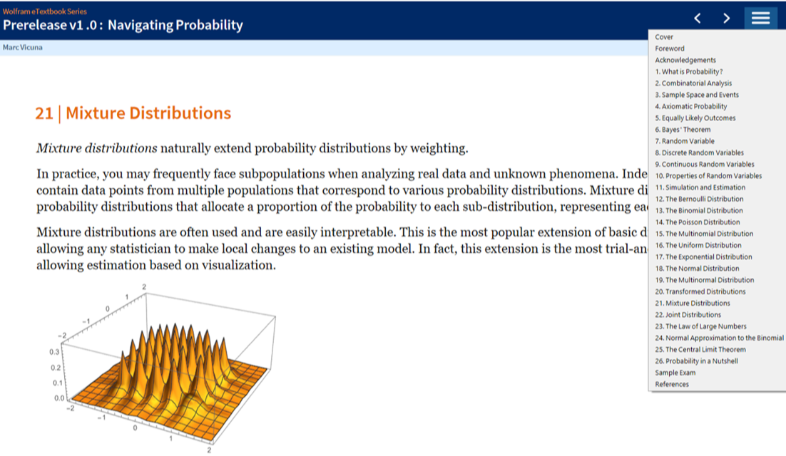
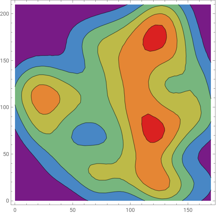
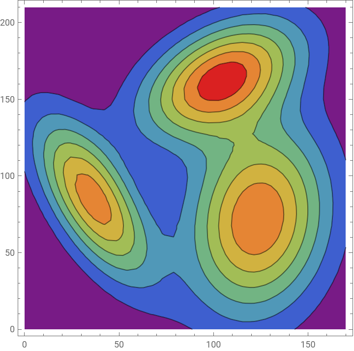
However, unlike most Introduction to Probability textbooks, it features a deeply modular and generalizable approach to construct any possible random variable with ease. Leveraging the extensive functionality of probability in Wolfram language, this short but deep textbook will uniquely enable you to generate random variables that accurately model any randomness you may encounter. Using Wolfram language, you’ll be able to create random variables as easily as you can visualize, analyze or simulate them.
In[]:=
TableContourPlotPDF[dist,{x,y}],{x,0,170},{y,0,210},,{dist,{myrtlesDist,GMMdist}}
Out[]=
,
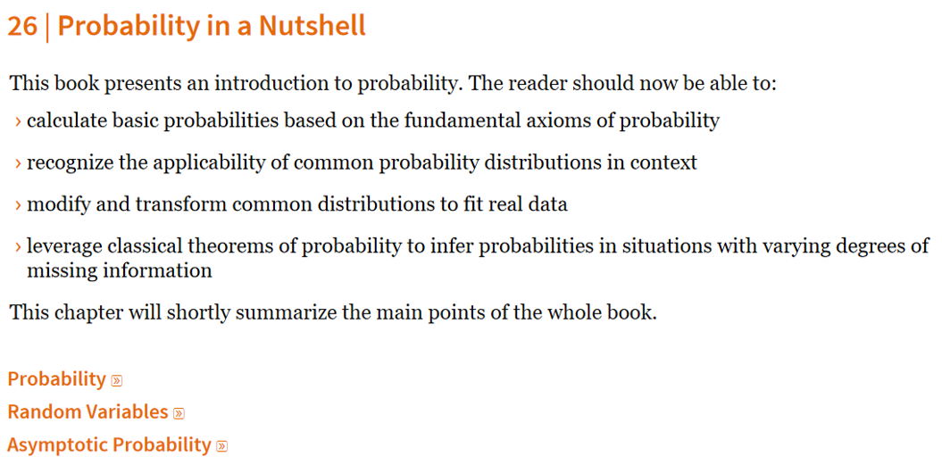
Of course, if it’s practice you’re seeking, deep exercises with complete solutions, as well as a sample exam and a short summary of the entire course (Probability in a Nutshell) are available for you to use and gain understanding at your preferred pace.
This pre-release paves the way for content additions, corrections and refinements. If you have any feedback concerning this ebook, you are formally invited to let us know through the feedback form https://www.wolframcloud.com/obj/wolfram-media/prerelease/NavigatingProbability/feedback. Note that Navigating Probability is only the first of a trilogy, as our ebooks on Discrete Mathematics and Game Theory will be coming soon. If you are a professor or teacher looking for a desk copy when available, feel free to write in at publishing@wolfram.com.
Book Introduction
Book Introduction
The concept of the unknown closely relates to randomness. Most will initially associate random events with situations we do not understand well. Randomness is often seen as a problem to minimize, an evil to eradicate. In applied sciences, randomness can very rarely be eradicated. Many scientists eventually realize that removing randomness is as futile as catching the wind. There are contexts in which randomness has its place and, dare I say, is appreciated. The most well-known of these is games of chance. In these games, randomness is the mechanism that levels the playing field, giving anyone a chance to win. It is with the same enthusiasm that we aim to introduce probability theory.
By understanding probability, you can establish patterns of randomness that demystify random phenomena to a much greater degree. This knowledge is fundamental in most modern applied fields, such as engineering, medicine, chemistry, epidemiology, seismology, insurance, sales, investing, forecasting, machine learning, robotics, sports, and games. More than just understanding it, you will become able to generate carefully crafted randomness, using it to your advantage.
This book provides a comprehensive introduction to probability. It starts with preliminary knowledge of combinatorial and set theory. It covers all the main topics of an introductory textbook to probability, including axiomatic probability, Bayes’ theorem, well-known probability distributions, statistical metrics, and well-known asymptotic theorems. Furthermore, it also includes advanced topics, such as the history of probability, common probability assumptions, advanced statistical metrics and functions, multivariate named distributions, transformed distributions, mixture distributions, joint distributions, and copula distributions. Moreover, a particular effort was dedicated to the mathematical proofs of most of the theorems introduced throughout the book, allowing the reader to see both practical and theoretical motivations for the probability concepts.
This book introduces probability computationally using Mathematica: a comprehensive computational software for all aspects of mathematics and beyond. The code is written in Wolfram Language: a general-purpose high-level programming language, which means it is very easy to read and can solve problems across a broad range of subjects. As a learning tool, Mathematica facilitates understanding by handling all the difficult or tedious aspects of dataset manipulation, probability computation, and distribution approximation, allowing the learner to simultaneously focus on important concepts and think computationally.
Please note that this book is not meant to be only read; it can be watched, practiced, and studied so that probability may not only be a topic you know about but also a skill you master. The reader will be exposed to the capabilities of Mathematica and will appreciate its power to work with larger datasets, visualize complex concepts, and think computationally. Dedicated Mathematica functions can quickly execute tedious calculations, allowing the reader to avoid getting bogged down with complicated sums and integrals (on which probability theory tends to rely heavily) and to focus on higher-level abstractions.
As mathematicians and statisticians, we hope our passion for games of chance transpires and our appreciation for the inexhaustible versatility of applied probability. This book is not just a set of theorems, proofs, and applications, but a stepping stone towards success in statistics and exploring the unknown. It will inspire you to achieve such mastery and drive you towards success.
Good luck!
The Wolfram Mathematical Computation Team
April 21, 2025
The Wolfram Mathematical Computation Team
April 21, 2025
Below is a sample chapter from the book
10 | Properties of Random Variables
10
| Properties of Random VariablesChapter 8 shows that many useful characteristics of probability distributions can be expressed using a single concept of expectation: the sum or integral of all values under some function weighted by their corresponding probability. This chapter unveils the power of expectation, as we discover that all the properties of random variables (RVs) are derived from expectation.
But what is expectation? As random variables are the mathematical formulation of random events, expectation is the mathematical formulation of the behavior we expect from these random events.
Just like the cat expects the plant to grow into a delectable flower, one should expect a list of behaviors from an event and its random variable. These behaviors can be calculated using expectation and the random variable’s PDF.

Mean
Mean
The () is the expected value of a random variable; it is also known as the average. It corresponds to the sum of all its values weighted by their corresponding probability.
μ
Formally, the mean is defined as the expectation of :
X
μ=E[x]
∑
x
∫xP(x)xdefinestheexpectationofcontinuousrandomvariables
Example 1
Example 1
The wait for customer service follows the probability density function (PDF) where . What is its mean?
2
-2x
e
0<x<∞
Solution:
Solution:
Build the probability distribution:
distE=ProbabilityDistribution[2E^(-2x),{x,0,Infinity}]
ProbabilityDistribution2,{x.,0,∞}
-2x.
Use either or :
{Expectation[x,xdistE],Mean[distE]}
,
1
2
1
2
This may also be done by the integral definition:
∞
∫
0
-2x
e
Integrate[x2E^(-2x),{x,0,∞}]
1
2
Variance
Variance
The () is the squared expected variation, and the () is its root. This metric helps gauge the distance away from the mean one may expect from a random event with a given probability of certainty. A large variance may indicate the instability of an event, while a small variance indicates its stability.
2
σ
σ
Due to Chebyshev’s Inequality, which will be explained in Chapter 23, one can be certain that most of the simulated values of a random event are at most one standard deviation away from the mean.
Formally, the variance is defined as the expectation of :
2
(X-μ)
2 σ |
2
(x-μ)
∑
x
2
(x-μ)
∫P(x)xdefinesthevarianceforcontinuousrandomvariables
2
(x-μ)
Example 2
Example 2
The wait for customer service follows the probability density function (PDF) where . What is its variance and standard deviation?
2
-2x
e
0<x<∞
Solution:
Solution:
For the variance, use either or :
{Expectation[(x-Mean[distE])^2,xdistE],Variance[distE]}
,
1
4
1
4
This may also be done by the integral definition:
∞
∫
0
2
(x-1/2)
-2x
e
Integrate[(x-1/2)^2*2E^(-2x),{x,0,∞}]
1
4
This may also be done by the integral definition by taking the square root of:
Expectation of Sums
Expectation of Sums
In the case of the addition of constants, the expectation of adding a constant to a random variable is equivalent to adding the constant to the expectation of that random variable:
This may be proven in the discrete case:
And in the continuous case:
Similarly, in the case of constant multiplication, the expectation of a constant multiplying a random variable is equivalent to a constant multiplying the expectation of that random variable:
This may be proven in the discrete case:
And in the continuous case:
In the case of the addition of two random variables, the expectation of the sum of two random variables is equivalent to the sum of the expectations of those random variables:
This may be proven in the discrete case:
And in the continuous case:
By induction, this principle may be applied to any number of random variables.
Example 3
Example 3
Solution:
Solution:
Build the probability distribution for each phase:
In the case of the product of two random variables, the expectation of the product of two random variables is equivalent to the product of the expectations of the random variables:
This may be proven in the discrete case:
And in the continuous case:
Variance of Sums
Variance of Sums
The natural extension of the expectation of sums is the variance of sums.
Assuming pairwise independent random variables, the variance of sums of random variables can be defined as:
However, if there are dependent pairs of random variables, the variance definition is modified to be:
Example 4
Example 4
Solution:
Solution:
Build the probability distributions for each phase:
The covariance between phases is:
Covariance
Covariance
Covariance is a measure of the relationship between two random variables. It is defined as:
As proven here:
As proven here:
As proven here:
Notice that the covariance between two or more random variables may be measured in many ways. To be complete, many use the covariance matrix to express covariance, which exhaustively enumerates all possible combinations of random variables for covariance. For two random variables, the covariance matrix is listed as follows:
Example 5
Example 5
Solution:
Solution:
Correlation
Correlation
The interpretation of covariance depends on the domain of random variables. The normalization of covariance, also known as correlation, may correct this.
By definition, correlation is the standardized degree to which two or more quantities are linearly associated:
You can infer some understanding from its values:
◼
1 implies a proportional dependency.
◼
−1 implies an inversely proportional dependency.
◼
0 implies a lack of correlation, also known as uncorrelated.
Of course, getting a correlation of exactly -1, 0 or 1 is rare. A correlation “close” to -1 will indicate an inversely proportional relationship, a correlation “close” to 0 will indicate independent random variables, and a correlation “close” to 1 will indicate a proportional relationship.
Empirically, correlation is often the main tool used to determine if random events are independent, where a low enough correlation may justify the independence assumption.
Moreover, many fields using statistics characterize the strength of a relationship between two random variables using the absolute value of the correlation. Many domains have their own definition of what constitutes independence, a weak relationship, a moderate relationship, or a strong relationship.
Example 6
Example 6
Solution:
Solution:
Moments
Moments
Computing moments is particularly useful when simplifying expectation expressions algebraically. Indeed, most of the expressions within an expectation expression are polynomials, and any term of that polynomial may be inferred from the moment of corresponding degree:
Multiple types of moments distinguish themselves from raw moments, most importantly, central moments, factorial moments, standardized moments and sample moments.
Central moments are defined as raw moments that are centered on the mean:
This change allows central moments to be location-invariant, leading to a better variability assessment.
Many useful statistical measures of distribution are built on moments. The most famous raw moment is the first, also known as the mean.
Example 7
Example 7
Solution:
Solution:
Build the probability distribution:
More Moments
More Moments
Moreover, variance is by definition equivalent to the second central moment:
Example 8
Example 8
Solution:
Solution:
Build the probability distribution:
A positive skewness would indicate an asymmetry where most probability is on the left of the mean.
A negative skewness would indicate an asymmetry where most probability is on the right of the mean.
Example 9
Example 9
Solution:
Solution:
Build the probability distribution:
A high kurtosis indicates a high concentration of data around the peak and tails.
A lower kurtosis indicates a lower concentration of data around the peak and tails.
Example 10
Example 10
Solution:
Solution:
Build the probability distribution:
Moment-Generating Functions
Moment-Generating Functions
This is often very useful for algebraic computation, and just from the PDF of a distribution and its moment-generating function, most common statistical computations can be algebraically found.
Example 11
Example 11
Solution:
Solution:
Build the probability distribution:
Conditional Expectation
Conditional Expectation
Why can the expectation operation accurately predict any random variable?
One branch of statistics studies the notion of estimator. This has led to a very interesting and useful fact about estimators, most notably the “best” estimator.
Summary
Summary
◼
The mean is the weighted average of all the values of a random variable, and it is the first raw moment. It is also the best estimator.
◼
The variance helps gauge the distance away from the mean random events may have, that is, the dispersion of the distribution. This idea can be extended to more than one random variable, where the covariance and correlation measure the strength of the relationship between random variables.
◼
Expectation has many identities, which facilitates its algebraic computation.
◼
More statistical metrics may be computed algebraically based on their PDF, raw moment generating function and central moment generating function.
Exercises
Exercises
2
.Find the mean, variance, skewness, and kurtosis of your distribution.
CITE THIS NOTEBOOK
CITE THIS NOTEBOOK
Introduction to Probability now available as a prerelease E-book!
by Marc Vicuna
Wolfram Community, STAFF PICKS, February 10, 2026
https://community.wolfram.com/groups/-/m/t/3637932
by Marc Vicuna
Wolfram Community, STAFF PICKS, February 10, 2026
https://community.wolfram.com/groups/-/m/t/3637932