In[]:=
Quit
In[]:=
PrependTo[$Path,DirectoryName[NotebookDirectory[],2]];
In[]:=
<<AmpRed`
************ AmpRed ************
********** Version 1.1 **********
Author: Wen Chen (chenwenphy@gmail.com)
In this notebook, we calculate the anomalous magnetic moment of the electron by using AmpRed.
By default, AmpRed uses such a convention that the prefactor of each fold of loop integration is Pi^(-D/2). To get the physical result, we need to further add a prefactor of (4*Pi)^(-D/2) by setting the option:
In[]:=
SetOptions[AmpRed,"LoopPrefactor"(4*Pi)^(-D/2)];
For simplicity, we put the electron on shell and use the Lorenz gauge:
In[]:=
SetKinematics[{p[1]}{k[1],k[2]},{m}{m,q}];m=1;SetOptions[PolarizationVector,"Transverse"True];
In[]:=
LaunchKernels[8];
We generate the vertex diagram and the corresponding amplitude by using ARQgraf:
In[]:=
diag=ARQgraf[{"F"}{"F","V"},1,"Style""Diagram","Model""QED"];
The generated digram can be painted by using ARTikzFeynman:
In[]:=
Magnify/@ARTikzFeynman[diag]
Out[]=
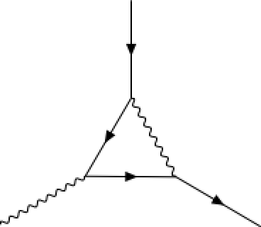
The corresponding amplitude is:
In[]:=
amp=ARQgraf[{"F"}{"F","V"},1,"Style""Amplitude","Model""QED"]/(I*EL)/.ELSqrt[4*Pi*α]/.{_ColourChain1,_ARCharge-1,_ARMassm};(*HereEListheQEDcouplingconstant.*)
One of the advantages of AmpRed is that it can decouple the loop integrals from the tensor structures with the latter untouched:
In[]:=
amp1=ToFeynmanInt[amp,l[1]]//AlphaParametrize;
Here ToFeynmanInt expresses an amplitude in terms of Feynman integrals (represented by FeynmanInt[...] or TensorInt[...]), and AlphaParametrize parametrizes Feynman integrals with the result expressed in terms of AlphaInt[...].
The tensor structures can be simplified by using ContractLI and SpinorChainSimplify:
In[]:=
amp2=SpinorChainSimplify[amp1//ContractLI];
We extract the independent tensor structures by using the function ExpandAR:
In[]:=
amp3=ExpandAR[amp2/.Momentum[p[1]]Momentum[k[1]]+Momentum[k[2]]//MomentumExpand//ContractLI,SpinorChain|Pair];
As we can see, only the following two tensor structures survive:
In[]:=
ts=Cases2[amp3,HoldAR[__]]
Out[]=
HoldAR().u()·,HoldAR()..u()
u
k
1
p
1
k
1
ϵ
k
2
u
k
1
ϵ
k
2
p
1
The g-2 is proportional to the coefficient of the first tensor structure:
In[]:=
gm2=-Coefficient[amp3//Total,ts[[1]]]//Simplify
Out[]=
-16πα(D-2)--2,1,1,0,D-2+2(D-2)--2,2,0,0,D-2-2--1,1,0,0,D-3
I
1
D
2
I
1
D
2
I
1
D
2
Now we can evaluate the scalar coefficient numerically. Because g-2 is measured in the non-relativistic limit, we take q->0 (For simplicity, we can also set q=0 from the very beginning):
In[]:=
gm2n=epsSeries[AlphaIntEvaluateN[gm2,4,{q0}][[1]]]
Out[]=
0.1591549431α
which reproduces the well known one-loop result:
α
2π
For multi-loop corrections, to accelerate the calculation, some steps of the calculation can be modified. See the example notebooks “HiggsDecay_TwoLoop.nb” and “HiggsDecay_TwoLoop_QGRAF+FORM+KIRA.nb”.