In this short computational essay , we will discuss measurement-based quantum computing as an alternate model to quantum computing . We will show how simple rules of measurements to cluster states can be utilized to generate complex computations. Under certain conditions, we can represent an equivalent circuit for any graph that has subset of vertices(qubits) measured. Finally we will explore briefly with simple examples the measurement calculus, that is a more formal way to do measurement-based quantum computations that also proves is universal.
Special thanks to my colleagues from the Wolfram Quantum Computation Framework Team, Nikolay Murzin and Mads Bahrami for their advice and interesting ideas about this topic.
There are many good references , but the ones i consider very fundamental are :
Paclet Installation
Paclet Installation
Install and load the Wolfram Quantum Computation framework:
In[]:=
PacletInstall["https://wolfr.am/DevWQCF",ForceVersionInstall->True]
Out[]=
PacletObject

In[]:=
<<Wolfram`QuantumFramework`
Helper Definitions
Helper
Definitions
Equatorial basis definition :
In[]:=
eb=QuantumBasis<|Interpretation["",0]->{1,Exp[Iθ]}",1]->{1,-Exp[Iθ]}
θ
+
2
,Interpretation["θ
-
2
|>,"Parameters"->θ;M operator for doing measurements in CME pattern:
In[]:=
m=QuantumMeasurementOperator[Cos[θ]QuantumOperator["X"]+Sin[θ]QuantumOperator["Y"],"Parameter"->θ];MM=FullSimplify[m["DiscardExtraQudits"],0<=θ<2Pi];M[θ_]:=QuantumOperator[QuantumOperator[Inverse[m[θ]["Eigenbasis"]["Matrix"]]]@MM[θ],"Label"->"Measurement"[m[θ]["Label"]]];
Graph states and fundamental measurement lemma
Graph states and fundamental measurement lemma
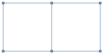
A graph or cluster state is a highly entangled quantum state , which has a direct representation from a mathematical graph . The edges of the graph represent the entanglement between qubits with a controlled Z operator . The graph state is defined as
G
E
G 〉
〉
0
G
:=
∏
(j,k)ϵE
C
j,k
〉
0
G
+〉
+〉
⊗n
+〉
In[]:=
g=GridGraph[{2,3},ImageSize->Small]
Out[]=
The QuantumFramework supports graph states:
In[]:=
QuantumState["Graph"[g]]
Out[]=
QuantumState

Measurement based quantum computing (MBQC) is a universal computing paradigm that makes use of these states, equatorial basis ) measurements are really important in MBQC because of a fundamental lemma. Let the state =⊗ with ψ 〉 an arbitrary one qubit state, and apply an equatorial measurement to the first qubit. If the outcome is then the state of the second qubit is
(|±α〉=1/±
2
|0 〉
α
1〉
| Ψ 〉
C
12
(
|ψ 〉
1
|+ 〉
2
)
M(α)
m
〉
ψ
2
=
H
m
Z
RZ
ψ 〉
m
X
H(α)
RZ
ψ 〉
Define the ψ state:
In[]:=
ψ=QuantumState["RandomPure"];
Define the Ψ state:
In[]:=
Ψ=QuantumOperator["CZ"]@QuantumTensorProduct[ψ,QuantumState["+"]];
Equatorial state projection:
In[]:=
projected=Through[(SuperDagger/@eb[α]["BasisStates"])[Ψ]];
Transformation of the measurement lemma:
In[]:=
transformed=Table[(QuantumOperator["H"]@(QuantumOperator["Z"]^m)@QuantumOperator["RZ"[α]]@ψ),{m,0,1}];
Verify the equality comparing density matrices, factor is included because the projection makes the state not normalized:
2
In[]:=
Chop@FullSimplifyMapThreadNormal[#1["DensityMatrix"]]-Normal[#2["DensityMatrix"]]&,
2
projected,transformed,α∈RealsOut[]=
{{{0,0},{0,0}},{{0,0},{0,0}}}
This lemma can be used in bigger cluster states employing more measurements to implement diverse circuits of any number of qubits. But we can observe that depending of the measurement outcomes Pauli corrections are needed to get the circuit exactly.
Equivalence of measuring cluster states and implementing circuits
Equivalence of measuring cluster states and implementing circuits
We will verify symbolically that doing measurements to a graph state has an equivalent circuit representation. In these examples is assumed all the equatorial basis measurements gave as outcome the state (m = 0) , because in that case Pauli corrections are not needed. Usually in experimental photonic MBQC corrections cannot be performed and the desired transformation is post-selected.
θ
+
In[]:=
$Assumptions=Element[{α,β,γ},Reals];
(3)Lcluster
(3)
L
Qubits 1 and 2 are measured
In[]:=
g=Graph[{1<->2,2<->3},VertexLabels->Automatic]
Out[]=

We can use graph states directly using the QuantumFramework:
In[]:=
state=QuantumState["Graph"[g]];
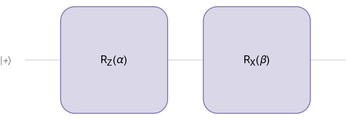
Consider the circuit:
In[]:=
q=QuantumCircuitOperator[{"RZ"[α],"RX"[β]}];q["Diagram","WireLabels"->{"+〉"}]
Out[]=
Verifying the equality:
In[]:=
result1=4(QuantumOperator[eb[β]["BasisStates"][[1]]["Dagger"],1]@QuantumOperator[eb[α]["BasisStates"][[1]]["Dagger"],1]@state)["DensityMatrix"]//Normal;
In[]:=
result2=(q[QuantumState["Plus"]])["DensityMatrix"]//Normal;
In[]:=
FullSimplify[result1-result2]
Out[]=
{{0,0},{0,0}}
(4)L state
(4)
L
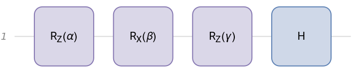
Qubits 1, 2 and 3 are measured. This configuration can be used to implement an arbitrary single qubit gate
In[]:=
g=Graph[{1<->2,2<->3,3<->4},VertexLabels->Automatic]state=QuantumState["Graph"[g]];
Out[]=

Projectors:
In[]:=
projs=eb[#]["BasisStates"][[1]]["Dagger"]&/@{α,β,γ};
In[]:=
q=QuantumCircuitOperator[{"RZ"[α],"RX"[β],"RZ"[γ],"H"}];q["Diagram"]
Out[]=
In[]:=
result1=8RightComposition[Sequence@@projs][state]["DensityMatrix"]//Normal;
In[]:=
result2=ComplexExpand[q[QuantumState["Plus"]]["DensityMatrix"]//Normal];
In[]:=
%-%%//Simplify
Out[]=
{{0,0},{0,0}}
(4)Horseshoecluster
(4)
Horseshoe
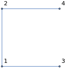
Qubits 1 and 2 are measured
In[]:=
g=EdgeDelete[GridGraph[{2,2},VertexLabels->Automatic],{4<->3}]state=QuantumState["Graph"[g]];
Out[]=
In[]:=
q=QuantumCircuitOperator[{"CZ","RZ"[α],"RZ"[β]->2,"H"->{1,2}}];
In[]:=
q["Diagram","WireLabels"->{Style["|+〉",14],Style["|+〉",14]}]
Out[]=
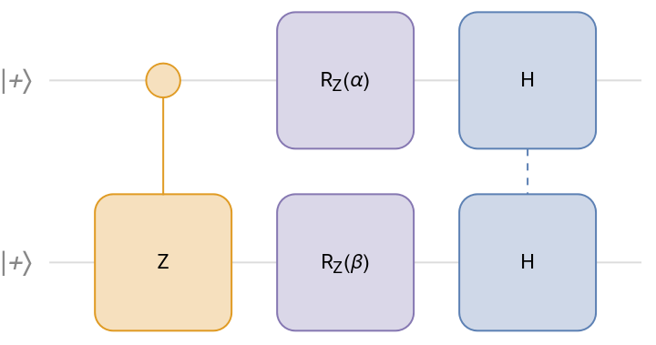
In[]:=
projs=eb[#]["BasisStates"][[1]]["Dagger"]&/@{α,β};
In[]:=
result1=4RightComposition[Sequence@@projs][state]["DensityMatrix"]//Normal;
Qubits 1 and 2 are measured
Qubits 1 and 2 are measured
Some extra example
Some extra example
Qubit 3 will be measured
Graph to Circuit
Graph to Circuit
From the previous examples , it is clear that is possible to automate the process of building a circuit from measuring certain qubits of a graph state. To have a direct algorithm it is required the graph follows the methodology of Experimental One-Way Quantum Computing , such that the graph is arranged in a grid-like fashion following the flow of information.
Examples
Examples
Let’s see some generated circuits using the function:
Invalid input because the way the graph is arranged would represent a 1 qubit circuit but is not
CME patterns in MBQC
CME patterns in MBQC
There is also a different approach to one-way quantum computing that is based entirely on a semantic calculus of patterns. The calculus incorporates a rewrite system of rules and algebra of pattern composition , patterns can also be extended with tensor product. The most fundamental types of patterns are called CME patterns that are composed of the following commands:
Linear chain teleportation
Linear chain teleportation
For example in the case of 3 qubits, with computation space {1,2,3} with inputs{1} and outputs {3}, it is possible to show the following pattern implements the teleportation protocol:
Check the equality:
CNOT gate
CNOT gate
General one qubit rotation
General one qubit rotation
A general XZX rotation can also be described with a pattern of computational space {1,2,3,4,5} with inputs {1} and outputs {5} :
Slight modification to M operator for labeling purposes:
Verify the pattern:
CITE THIS NOTEBOOK
CITE THIS NOTEBOOK
Measurement based quantum computing: equatorial measurement rules, equivalent circuits and patterns
by Bruno Tenorio
Wolfram Community, STAFF PICKS, May 22, 2024
https://community.wolfram.com/groups/-/m/t/3180183
by Bruno Tenorio
Wolfram Community, STAFF PICKS, May 22, 2024
https://community.wolfram.com/groups/-/m/t/3180183