Introduction
Introduction
Classically, cellular automaton run either on linear sequences of tiles or flat two dimensional grids. A natural generalization is to consider cellular automaton on grids that twist and bend in various ways. This project aims to explore the behavior of totalistic cellular automaton on surfaces including the sphere, the Möbius Strip, the Klein Bottle, the Real Projective Plane, and the genus-2 surface. The primary goal is to understand how the topological invariants of a grid correlate with attributes of CA evolution such as the periodicity of certain CA configurations under specified transition rules. The motivation is to better understand the global properties of local rules. Additionally, the results of this project demonstrates, as a proof of concept, that it might be possible to utilize CA as a computational tool to understand the topological properties of a given surface.
Surface Discretization
Surface Discretization
In order to run CA on surfaces, we tessellate the surfaces with squares. This is done by taking a standard grid graph with diagonal edges added, and gluing together the boundaries of the grid in various ways by adding in extra edges. The exception is with the genus-2 surface, where an octagon grid was used.
Each vertex of the graph represents a square tile on the tessellated surface, with undirected edges identifying adjacent tiles. This produces 8-regular graphs for the Torus, the Klein Bottle, and the Real Projective plane, and graphs with all but a few vertices of degree 8 for the Möbius strip, the Sphere, and the genus-2 surface. The advantage of this approach is that it allows us to easily standardize the number of vertices and edges in the graphs generated by surfaces.
Each vertex of the graph represents a square tile on the tessellated surface, with undirected edges identifying adjacent tiles. This produces 8-regular graphs for the Torus, the Klein Bottle, and the Real Projective plane, and graphs with all but a few vertices of degree 8 for the Möbius strip, the Sphere, and the genus-2 surface. The advantage of this approach is that it allows us to easily standardize the number of vertices and edges in the graphs generated by surfaces.
◼
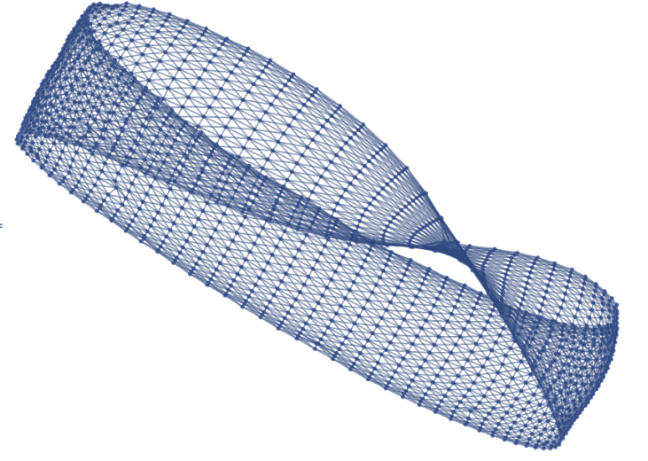
Möbius Strip constructed from a 20 by 80 grid
◼
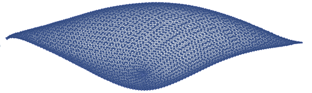
Football (or sphere) constructed from a 60 by 60 grid
◼
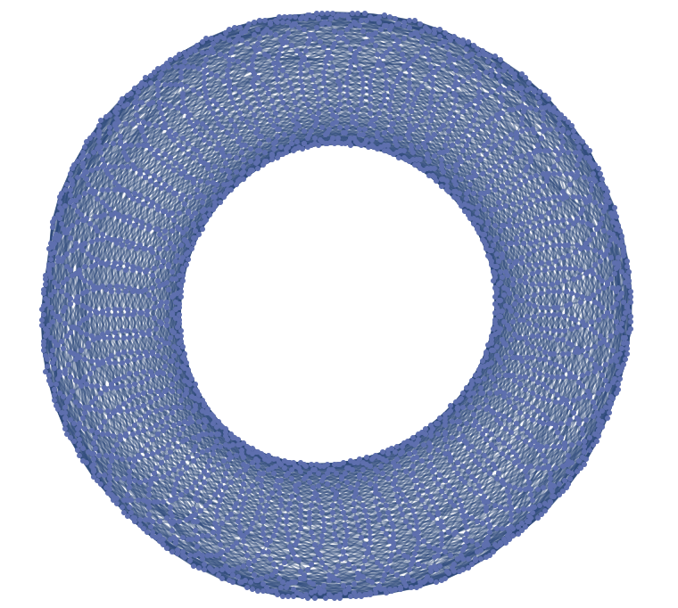
Torus constructed from a 60 by 60 grid
◼
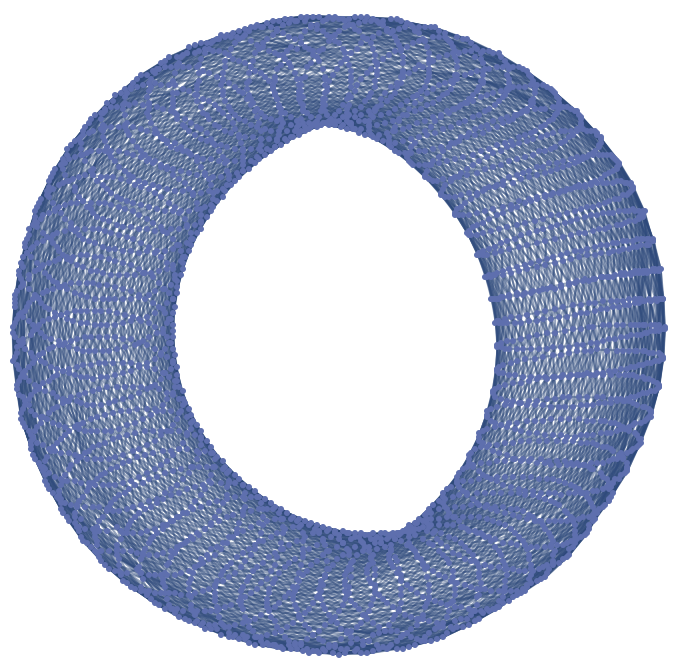
Klein Bottle constructed from a 60 by 60 grid. It is the torus with a twist. No pun intended.
◼
Real Projective Plane constructed from a 60 by 60 grid
◼
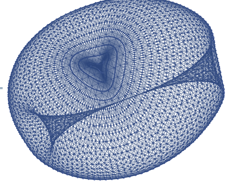
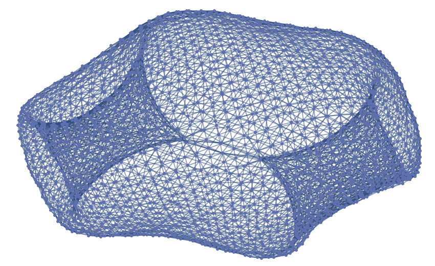
Genus-2 surface constructed from an octagon grid with side lengths of 20. I am hesitant to call this a double torus because it doesn’t resemble one.
CA on Graphs
CA on Graphs
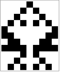
Having constructed the graph representations of the surfaces we’re interested in, we are now ready to run cellular automaton on them. To illustrate how this works, consider the one-dimensional CA rule 90. With the built in CellularAutomaton function, We can run rule 90 on a cyclic list of length 9 for 10 time steps, starting with a single live cell:
In[]:=
CellularAutomaton[90,{0,0,0,0,1,0,0,0,0},10]//ArrayPlot
Out[]=
We can reproduce the same iteration on a cyclic graph of order 9:
In[]:=
animateOnGrid[CycleGraph[9],{0,0,0,0,1,0,0,0,0},{1},{1},10]
Out[]=
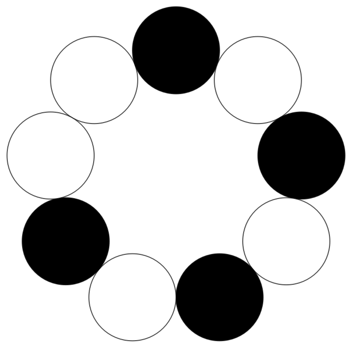
The first argument of the function specifies the graph on which the CA is ran--this can be any arbitrary graph. The second argument admits a list of initial conditions, whose length needs to be the same as the order of the graph. The initial conditions in the list are associated with the vertices of the graph in the order of VertexList[ ]. The Third and fourth argument specifies the transition rule in the same way that “GrowthSurvivalCases” does for CellularAutomaton[ ].
A more sophisticated example is running Conway’s Game of Life on a 10 by 10 grid, with random initial conditions:
A more sophisticated example is running Conway’s Game of Life on a 10 by 10 grid, with random initial conditions:
In[]:=
g=diagonalGridGraph[10,10];initialCondition=RandomInteger[{0,1},100];animateOnGrid[g,initialCondition,{2,3},{3},10]
Out[]=
State Transition Diagrams
State Transition Diagrams
One brute-force method to analyze the differing behavior of CA on different surfaces is computing state transition diagrams. These are graphs where each distinct state on the grid is associated with a vertex, with a directed edge going from u to v if the grid state associated with u will evolve into the one associated with v in one time step under the specified transition rule. Below is the state transition diagram for the Game of Life on a 3 by 3 grid:
And this is the transition diagram for the same grid, but folded into a torus (actually, the complete graph of order 9 in this case):
One immediate observation we can make is that in the torus transition diagram, there are a lot more lone vertices looping back into themselves. These correspond to static board configurations, or “still-lifes”. While these diagrams are fun to look at, the biggest problem with them is that they are impossibly hard to compute for larger grid sizes. On a 10 by 10 grid, the number of possible states is:
That’s thirty zeros! This means we would have to restrict ourselves to incredibly small grids in order to run the computations in reasonable time. However, these grids, corresponding to very coarse tessellations, are insufficient to reflect the actual topology of the various surfaces. For example, the 3 by 3 Klein Bottle grid is the same as that of the torus:
Gliders and Spaceships
Gliders and Spaceships
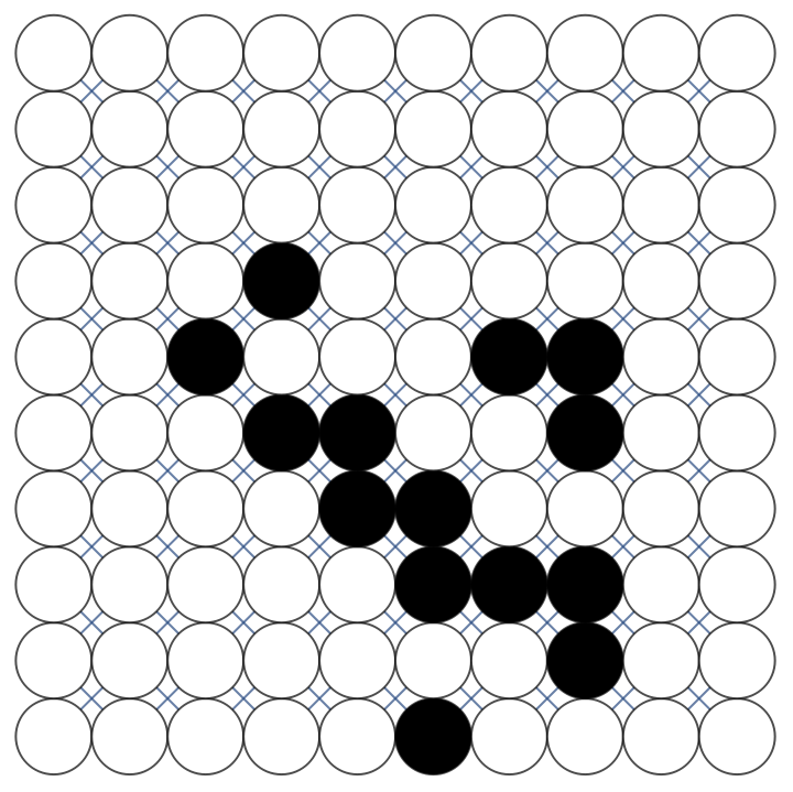
There is a way to sidestep the issue. On larger grids, the vast majority of possible states are irrelevant for our purposes. For instance, we should expect still-lifes to behave the same regardless of the global structure of the grid, since they remain localized. There is a very small subset of possible states that actually interact with the topology of the grid in interesting ways. For this project, I’ve focused on two particular types of constructs in the Game of life that are very mobile: gliders and lightweight spaceships.
◼
Gliders
This is an example of a glider on a 10 by 10 Klein Bottle. Gliders come in four orientations, each traveling in one of the four diagonal directions of the grid.
Because they move diagonally on the grid, when placed on a torus, they travel in a spiral-like path as shown above.
◼
Light weight spaceships
This is a light weight spaceship traveling on a genus-2 surface. Like gliders, they come in four different orientations. But the difference is that they travel horizontally and vertically.
When placed on the real projective plane, light weight spaceships move in seemingly erratic paths.
State Transition Diagrams for Gliders and Spaceships
State Transition Diagrams for Gliders and Spaceships
After limiting our scope to gliders and spaceships, computing state transition diagrams becomes much more manageable. The graphs in this section are generated by iterating every possible glider/starship on the grid for a given number of time steps.
20 x 20 standard grid, 30 iterations
20 x 20 standard grid, 30 iterations
The glider transition diagram above looks quite boring as expected, since all gliders are destined to hit the boundaries of the grid and become still-lifes.
Similar things happen to the spaceships:
20 x 20 Möbius Strip, 30 iterations
20 x 20 Möbius Strip, 30 iterations
The glider transition diagram for the Möbius strip exhibit similar characteristics as that of the flat grid.This is because gliders travel diagonally, hence they will eventually hit the boundaries of the surface as well:
However, since some of the the spaceships travel horizontally, they’re able to return to their starting locations eventually, as the cycles indicate, while the vertically traveling spaceships would still hit the boundaries of the surface, as the lines indicate:
30 x 30 Sphere, 40 iterations
30 x 30 Sphere, 40 iterations
The square tiling of the sphere will always result in singularities at the poles. Whenever a glider travels to one of the poles, it disappears entirely. These gliders trace out the rays in the star-shaped graph component below.
Similar behavior is observed for the spaceships:
30 x 30 Torus, 40 iterations
30 x 30 Torus, 40 iterations
There are two interesting things to point out about the glider and spaceship diagrams for the torus. First, there are 120 cycles in the glider transition diagram below--Exactly double the sum of the dimensions of the grid. This means that each inner vertex on the boundaries of the square grid in the construction of the torus uniquely determines a glider path around the torus, while other four each determine two. Moreover, since there are more ways to loop around a torus compared to the sphere due to their homology, there are also more cycles in both of the diagrams below compared to their counterparts for the sphere .
Additionally, there are also more cycles in the spaceship diagram below compared to the glider diagram above. This is because spaceships are able to travel around the meridians and the equators of the torus, but the gliders could only travel in spiral paths.
30 x 30 Klein Bottle, 40 iterations
30 x 30 Klein Bottle, 40 iterations
The number cycles in the glider diagram is exactly half of that of the torus. It is simply the sum of the dimensions of the square grid. The added twist of the Klein bottle merged paths around the torus in pairs.
For the spaceship diagram below, cycles of two different lengths are present. These correspond to the horizontally traveling spaceships whose paths on the torus were merged on the Klein Bottle, and the vertically traveling spaceships whose paths remained the same.
30 x 30 Real Projective Plane, 40 iterations
30 x 30 Real Projective Plane, 40 iterations
The glider transition diagram (top) and spaceship transition diagram (bottom) for the real projective plane looks very similar to those of the sphere, except that a few additional cycles appear. A tentative explanation is as follows: because the quotient map transforming the sphere into the real projective plane is also a double covering map, any closed path on the real projective plane either correspond to another closed path on the sphere, or a path between pairs of antipodal points, via the lifting property of covering maps. And it just so happens that not many gliders and spaceships pass through pairs of antipodal points on the sphere due to the way they travel, which would correspond to the few extra cycles in the diagrams below.
Comparison
Comparison
We can compute the graph union of glider/spaceship transition diagrams across different surfaces to visualize how the same initial conditions evolve along different paths due to the differing topology:
◼
Torus vs Klein Bottle, Gliders
◼
Torus vs Klein Bottle, Spaceships
◼
Real Projective Plane vs the Sphere, Gliders
◼
Real Projective Plane vs the Sphere, spaceships
Concluding Remarks
Concluding Remarks
This project focused mostly on the behavior of the Game of Life on a selection of topological surface, specifically the behavior of gliders and spaceships. Both qualitative and qualitative difference was observed between the periodicity of both gliders and spaceships across different surfaces, specifically with regards to closed paths. Future work may include exploring other self-propagating structures in the Game of Life, as well as experimenting with other types of transition rules, especially ones that aren’t totalistic--those rules are likely more sensitive to the non-Orientability of some surfaces.
Special thanks to my mentor Bradley K. for all the support, as well as Stephen for inspiring me to choose this project. To those in Team Computer Fun, it has been a pleasure working together with you, wish you all the best!
Special thanks to my mentor Bradley K. for all the support, as well as Stephen for inspiring me to choose this project. To those in Team Computer Fun, it has been a pleasure working together with you, wish you all the best!
Code
Code
CA iterator
CA iterator
Surface constructors
Surface constructors
Visualization
Visualization
Analysis
Analysis
Game of Life constructs
Game of Life constructs