This is an interesting - and important - topic, thanks for sharing!
“Case 3. CO2 emission (giga tons / year) increases quadratically. This reflects current economic development ...”
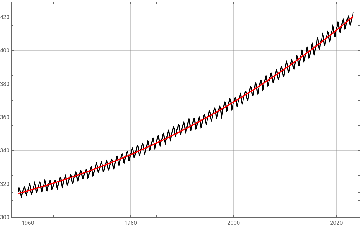
You may be right, but I am still not really convinced about that point. So I had a look into real world data - using the data from the famous Keeling curve (describing the accumulated CO2 concentration over time). From this a polygonal fit is done:
You may be right, but I am still not really convinced about that point. So I had a look into real world data - using the data from the famous Keeling curve (describing the accumulated CO2 concentration over time). From this a polygonal fit is done:
In[]:=
dataRaw=Import["https://scrippsco2.ucsd.edu/assets/data/atmospheric/stations/in_situ_co2/monthly/monthly_in_situ_co2_mlo.csv"];dataKeeling=TimeSeries[{DateObject[{#1,#2}],#3}&@@@dataRaw[[62;;-9,{1,2,9}]]];
In[]:=
Clear[t,c0,c1,c2,c3];model=c0+c1t+c2t^2+c3t^3;params=FindFit[dataKeeling,model,{c0,c1,c2,c3},t];
In[]:=
params//TableForm
Out[]//TableForm=
c0291.435 |
c12.3682× -9 10 |
c23.31829× -18 10 |
c31.18191× -27 10 |
So, we see that the third order coefficient is just tiny. But the fit seems to be reasonable:
In[]:=
(*comparison:measurementwithfitteddata*)month=QuantityMagnitude@UnitConvert[Quantity[1,"Months"],"Seconds"];{start,end}=AbsoluteTime@*dataKeeling/@{"FirstDate","LastDate"};fitdata=Table[{t,model/.params},{t,start,end,month}];DateListPlot[{dataKeeling,fitdata},ImageSize->Large,PlotStyle->{Black,{Thick,Red}},GridLines->Automatic]
Out[]=
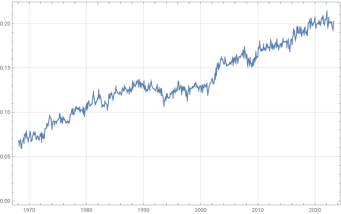
From these data one can also deduce the tendency of CO2 emission, which basically seems to be a first order function:
In[]:=
DateListPlot[Differences@MovingAverage[dataKeeling,120],GridLines->Automatic,ImageSize->Large]
Out[]=
Where am I wrong, do I see things too simple? Well - the tendency is alarming anyway!
Regards -- Henrik