CITE THIS NOTEBOOK: Animation of a Robert type 1 mechanism by David Balandra. Wolfram Community JAN 19 2023.
Spatial or planar mechanisms can be applied to solve repetitive tasks requiring reciprocating motion, movements following trajectories given by mathematical functions or, in general, an spatial movement. To create an optimal design of a mechanism, it is necessary to analyze and simulate its movement before prototype or construct it. The following code can be modified or adapted to analyze planar or spatial mechanisms.
Type 1 Robert Linkage
Type 1 Robert Linkage
Functions
Functions
In[]:=
Tx[x_]:=TranslationTransform[{x,0,0}][[1]];(*translationinxaxis*)Ty[y_]:=TranslationTransform[{0,y,0}][[1]];(*translationinyaxis*)Tz[z_]:=TranslationTransform[{0,0,z}][[1]];(*translationinzaxis*)Rx[θx_]:=RotationTransform[θx,{1,0,0}][[1]];(*rotationaroundxaxis*)Ry[θy_]:=RotationTransform[θy,{0,1,0}][[1]];(*rotationaroundyaxis*)Rz[θz_]:=RotationTransform[θz,{0,0,1}][[1]];(*rotationaroundzaxis*)T3D[V_]:={V[[1]],V[[2]],V[[3]]};(*transformsa4Dvectorintoa3Dvector*)
Parameters
Parameters
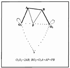
Figure1Type1RobertLinkage
In[]:=
l1=6;(*linkAB*)l2=2l1;(*linkA*)l3=l2;(*link*)l4=l3;(*linkAP*)l5=l4;(*linkPB*)(*=2l1*)
O
1
BO
2
O
1
O
2
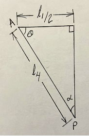
Figure2HalfsectionoftriangularlinkABP
In[]:=
θ=ArcCos;(*anglebetweenAPandAB*)α=ArcSin;(*anglebetweenAPandmidpointofAB*)
l1
2l4
l1
2l4
Kinematic Analysis
Kinematic Analysis
Position Equation
Position Equation
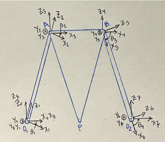
The position equation is obtained by describing the successive translations and rotations of a coordinate system following the mechanism geometry in a given fixed position.Figure 3 A coordinate System moving along the closed loop -A-B--.
O
1
O
2
O
1
The transformation matrices T1, T2 and T3 below give the positions and orientations of the coordinate system following the closed loop -A-B--. For example, the first movement, Ry[θ1], is a rotation around the axis, which transforms the -- coordinate system into --. As can be seen in Figure 3, all the y axes are directed into the page.
Note that the last-- coordinate system is in the same position and orientation as the initial -- coordinate system. This is mathematically reflected in the Objective Function 1 below, which comes from the condition of loop closure: P1=P2.
O
1
O
2
O
1
Y
0
X
0
Y
0
Z
0
X
1
Y
1
Z
1
Note that the last
X
8
Y
8
Z
8
X
0
Y
0
Z
0
In[]:=
Clear[θ1,θ2,θ3,θ4];T1=Ry[θ1].Tz[l2].Ry[θ2];(*position:jointA,orientation:xaxisalignedwithAB*)T2=Tx[l1].Ry[θ3];(*position:jointB,orientation:xaxisalignedwith*)T3=Tx[l3].Ry[θ4].Tx[-2l1];(*position:joint,orientation:xaxisalignedwith*)P1=T1.T2.T3;(*closedloop-A-B--followedbythecoordiantesystem*)P2=IdentityMatrix[4];(*conditionofloopclosure:P1=P2*)OF1=;(*ObjectiveFunction1writtenasnon-linearleastsquares*)
BO
2
O
1
O
1
O
2
O
1
O
2
O
1
4
∑
j=1
4
∑
i=1
2
(P1[[i,j]]-P2[[i,j]])
The transformation matrices T4 and T5 below give the positions and orientations of a coordinate system following the closed loop -A-P-B--. The angles θ and α are calculated from Figure 2.
O
1
O
2
O
1
In[]:=
T4=Ry[θ].Tx[l4];(*position:pointP,orientation:xaxisalignedwithAP*)T5=Ry[-π+2α].Tx[l5].Ry[θ+θ3];(*position:jointB,orientation:xaxisalignedwith*)P3=T1.T4.T5.T3;(*closedloop-A-P-B--followedbythecoordiantesystem*)OF2=;(*ObjectiveFunction2writtenasnon-linearleastsquares.Again,theconditionofloopclosure:P3=P2isapplied*)
BO
2
O
1
O
2
O
1
4
∑
j=1
4
∑
i=1
2
(P3[[i,j]]-P2[[i,j]])
In[]:=
OF3=OF1+OF2;(*Objectivefunctionofbothloops-A-B--and-A-P-B--*)
O
1
O
2
O
1
O
1
O
2
O
1
Initial Solution for the Position Equation
Initial Solution for the Position Equation
In[]:=
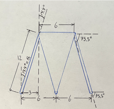
Clear[θ1,θ2,θ3,θ4];θ2=-ArcSin;(*entryangle,fromFigure4*)InitialSolution=FindMinimumOF3,θ1,ArcSin,θ3,ArcCos,θ4,-ArcCos,MaxIterations50(*initialguessesforθ2,θ3&θ4takenfromFigure4*)
l1
2l2
l1
2l2
l1
2l3
l1
2l3
The FindMinimum command is applied here as an optimization method which can solve the conditions of loops closure, P1=P2 and P3=P2, by minimizing the objective function OF3 only for the fixed position shown in Figure 4.
Complete Solution for the Position Equation
Complete Solution for the Position Equation
The FindMinimum command is iteratively applied above to solve the conditions of loops closure, P1=P2 and P3=P2, by minimizing the objective function OF3 for each of the 360 degrees of a complete revolution.
For each iteration, the initial values are taken from the immediately previous iteration.
For each iteration, the initial values are taken from the immediately previous iteration.
Animation
Animation
Animation Parameters
Animation Parameters
Animation left hand corner View
Animation left hand corner View
References
References
[1] Dr. Francisco Cuenca - UNAM University
[2] RIUTORT, Kevin T. Applied design and implementation of straight-line mechanisms. 1996. Tesis Doctoral. Virginia Tech
[3] https://youtu.be/jcAu0kBcptk Animation of a Type 1 Robert Linkage made with Wolfram Mathematica
[4] DEEPAK, Sangamesh R.; ANANTHASURESH, G. K. James Watt and his linkages. Resonance, 2009, vol. 14, no 6, p. 530-543.