Wolfram Cloud Page

Ever wondered what happens when you push thousands of vertices into a graphics engine?

GraphicsComplex

can write directly into GPU buffers with no overhead. Let's see how far we can take it.

Most high-level plotting functions hide the machinery behind a convenient interface. You call

ListPlot3D

, you get a surface — magic. But what if you want to control every vertex, every triangle, every color? What if you need to push 10³ animated points at least at 30 fps?

This is where

GraphicsComplex

comes in...

“Please take everything with a grain of salt, since this is only applicable to WLJS Notebook, but not to Wolfram Research products. Wolfram Mathematica might still heavily rely on a CPU pipeline.”

GraphicsComplex

mimics the interface of a low-level graphics API like OpenGL, WebGL, Vulkan, and others, since the GPU loves to eat vertices and polygon faces as separate dishes. Under the hood, it writes your vertex data directly into WebGL buffer attributes — later automatically synchronized with GPU memory buffers. The list of coordinates becomes a typed array

Float32Array

No intermediate conversions (at least for 3D), no SVG paths, no DOM nodes per point. It's as close to the metal as you can get from a digital notebook nowadays!

Find part 2 of this post here: https://community.wolfram.com/groups/-/m/t/3720773
Original Article: https://wljs.io/blog/graphicscomplex
The following code can be evaluated in WLJS Notebook.

Packed and Numeric Arrays

Numeric lists or tensors in Wolfram Language generated by

Table

Map

can become so-called packed arrays. For example, a manually constructed list is stored in memory as an array of pointers to some objects:

In[]:=

{1,2,3}//Developer`PackedArrayQ

Out[]=

False

However, if you generate it by a function with consistent types (only reals or only integers):

In[]:=

Table[i,{i,10}]//Developer`PackedArrayQ

Out[]=

False

Oops! Let's try bigger:

In[]:=

Table[i,{i,1000}]//Developer`PackedArrayQ

Out[]=

True

Here we go. In this case, this list is stored as a whole thing linearly in memory, which makes it especially efficient for storing data and processing.

In order to deoptimize it, we just need to break its homogeneity:

In[]:=

Table[If[i==1000,N[i],i],{i,1000}]//Developer`PackedArrayQ

Out[]=

False

Now we can compare it in size and time required for processing the data:

In[]:=

packed=Table[i,{i,1000}];unpacked=Table[If[i==1000,N[i],i],{i,1000}];

In[]:=

Quantity[ByteCount[packed],"Bytes"]//UnitSimplifyQuantity[ByteCount[unpacked],"Bytes"]//UnitSimplify

Out[]=

1037

128

KiB

Out[]=

189

Kib

Now the processing time with a simple function:

In[]:=

Quantity[Map[(##)&,packed];//AbsoluteTiming//First,"Seconds"]//UnitSimplifyQuantity[Map[(##)&,unpacked];//AbsoluteTiming//First,"Seconds"]//UnitSimplify

Out[]=

3.279

Out[]=

0.375

A cool thing, you can force Wolfram Kernel to keep your array as packed one with a given type and never unpack it using

NumericArray

wrapper:

In[]:=

packed//ByteCountNumericArray[unpacked,"SignedInteger64"]//ByteCount

Out[]=

8296

Out[]=

8296

NumericArray

gives you granular control over how your data is stored! This is amazing. If you know the boundaries of your data, it can save you a lot of resources:

In[]:=

NumericArray[unpacked,"SignedInteger16"]//ByteCount

Out[]=

2280

In WLJS, if you pass such an array explicitly or implicitly as a packed array to

GraphicsComplex

, it will be copied akin to

memcpy

directly to the corresponding typed array of JavaScript on our frontend. For example,

"SignedInteger16"

becomes an

Int16Array

view to

ArrayBuffer

. This is a key ingredient to performance and pays off extremely for

Image

and

Raster

primitives as well.

GraphicsComplex

The structure is simple:

GraphicsComplex[{pt1,pt2,...},primitives,attributes]

Coordinates given as integers

primitives

are replaced by the actual vertex

pti

. This separation of geometry data from topology is exactly how every modern graphics API works.

Starting simple: 2D

Let's start with a single triangle. Three vertices, one polygon:

In[]:=

Sequence[GraphicsComplex[{{-1,-1},{1,-1},{1,1}},Polygon[{1,2,3}],VertexColors->{{1,1,0},{0,1,1},{0,1,1}}],"Controls"->False,ImageSize->250]//Graphics

Out[]=

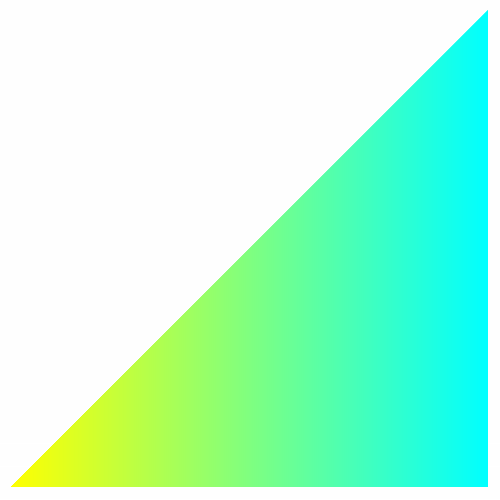
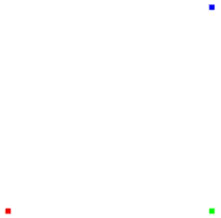
That gradient isn't computed on the CPU — the vertex colors are interpolated by the GPU's rasterizer, just like in any shader pipeline. You can do the same with points:

In[]:=

Sequence[GraphicsComplex[{{-1,-1},{1,-1},{1,1}},Point[{1,2,3}],VertexColors->{{1,0,0},{0,1,0},{0,0,1}}],"Controls"->False,ImageSize->250]//Graphics

Line

and

Arrow

are also supported, though they don't use hardware acceleration.

Polygon

and

Point

are where the GPU really shines.

Automatic triangulation

As you know, for GPU only triangles exist. Therefore if you provide something to

Polygon

with a face containing more than 3 indices it might use some power of CPU to triangulate the mesh:

In[]:=

Graphics[{GraphicsComplex[CirclePoints[0.7,50]//N,{LightBlue,Polygon[Range[1,50]],Red,Point[Range[1,50]]}]},PlotRange->{{-1,1},{-1,1}},"Controls"->False,ImageSize->250]

In this example, we have a polygon of 50 vertices. This might not be optimal for the case if indices change over time (animated), since then the data will be unpacked and reprocessed by JavaScript on the frontend. But for static graphics, this is the way to go.

Vertex Colors

For best performance, provide

VertexColors

as a plain

{{r,g,b}, ...}

list rather than symbolic colors like

Red

Hue[...]

. This avoids the overhead of converting color expressions on every frame:

In[]:=

v={{1,-1},{1,1},{-1,-1}};Graphics[{GraphicsComplex[v,Polygon[{1,2,3}],VertexColors->{Red,Blue,Green}]}]

VertexColors->{{r1,g1,b1},{r2,g2,b2},...}

img=ImageResize[ExampleData[{"TestImage","House"}],Scaled[1/4]];Graphics[{Texture[img],GraphicsComplex[{{-1,-1},{1,-1},0.2{1,1},{-1,1}},Polygon[{1,2,3,4}],VertexTextureCoordinates->{{0,1},{0,0},{1,0},{1,1}}]},"Controls"->False,ImageSize->250]

Or let the engine figure out the mapping automatically:

How to update things

Fixed indices

However, this is quite boring. Let's add some colors:

Here is a catch:

Let's update colors as well:

Going bigger

Let's try more vertices:

◼

animation goes as fast as possible;

◼

the next cycle starts only after the previous one is fully finished;

◼

update is in sync with GPU / window / OS refresh.

Now what if we push it further and animate 2500 dancing points?

This demo is based on the original work of Simon Woods "Dancing with friends and enemies: boids' swarm intelligence"

We did exactly what we discussed regarding packing colors and vertices to the same symbol. This also requires less data transfer calls. You can find, that the symbol itself is not packed array, but its parts are.

Dynamic topology: updating everything

We start from the indices and try to change it in real-time:

You don't need to worry about GPU buffer management. If the data does not fit, WLJS reallocates a bigger buffer (2x the requested size) and lets you use it automatically.

Going Bigger

Here's a 2D mesh with orbiting holes that dynamically removes and adds triangles, mutating indices, colors, and vertices as is usually done in games or 3D software — a full update cycle:

Of course, we can't just remove triangles from the given positions. In this particular example, it is done by subdividing the edges into much smaller triangles, avoiding sharp edges.

We hope you can find many great applications for this primitive we implemented. See you in the next part, where we will explore the 3D version of it.

Bonus: Ideal Gas Simulation

The rest is for the dessert

“Inspired by Jon McLoone (2007) Simulation of a Simple Gas Pressure Model”

Here is a simple two-dimensional toy model of the ideal gas. A collection of particles moves inside a square container, bounces elastically from the walls, and the simulation counts how often those wall collisions happen. The model is deliberately simple: particles do not collide with one another, and the temperature is represented by the step size of their motion (kinetic energy). All of this just to prove:

CITE THIS NOTEBOOK

Real-time GPU rendering via local JavaScript engine. Part 1
by Kirill Vasin
Wolfram Community, STAFF PICKS, May 21, 2026
https://community.wolfram.com/groups/-/m/t/3720274